Page 1
UNIVERSITÀ DEGLI STUDI DI SALERNO
FACOLTÀ DI INGEGNERIA
CORSO DI LAUREA IN INGEGNERIA CIVILE
Tesi di Laurea in
Tecnica delle Costruzioni
A NEW TIMOSHENKO-BASED ANALYTICAL
MODEL FOR STEEL-CONCRETE COMPOSITE BEAMS
IN PARTIAL INTERACTION
RELATORE CANDIDATO
Prof. Ing. Ciro Faella Giuseppe Di Palma
CORRELATORE Matr. 163/000542
Dott. Ing. Enzo Martinelli
Anno Accademico 2007/2008
Page 2
In the Name of Allah, the Most Gracious, the Most Merciful
« Read!, In the Name of your Lord Who has created,
He has created man from a clot ,
Read!, and your Lord is the Most Generous,
Who has taught by the pen,
He has taught man that which he knew not » .
The Noble Qur’an, Surat XCVI, 1‐5
Page 4
Ai miei cari Genitori:
senza i loro sacrifici, la loro pazienza e il loro incoraggiamento
questa Tesi non sarebbe stata mai scritta.
Grazie.
Page 6
i
Sommario
1.Introduction 1 1.1State of the art 1
2.A Timoshenko‐based model for composite beams in partial interaction 7 2.1Key geometric and mechanical properties of the composite cross section 7 2.2Model equations 8
2.2.1 Equilibrium equations 8 2.2.2 Constitutive laws 11 2.2.3 Global equilibrium equation 13 2.2.4 Compatibility equation throughout the interface 13 2.2.5 Equilibrium equation throughout the interface 14 2.2.6 Stress‐strain law for shear connection 15
3.Outline of the governing equations 16 3.1The system of three equations in three unknown functions 16 3.2Displacement formulation 18
3.2.1 Deducing the problem dimensions 19 3.2.2 Differential equation in terms of deflection 22 3.2.3 Deriving the other parameters 25
3.3Extended Newmark’s equation in terms of curvature 30
4.Solution in the elastic range 36 4.1Composite beam under axial force 36 4.2Composite beam in bending 37
4.2.1 Non‐redundant beams in bending 40 4.2.2 Boundary conditions for non‐redundant beams 42 4.2.3 Redundant beams in bending 47 4.2.4 Boundary conditions for redundant beams 48
Page 7
Giuseppe Di Palma 163/000542
ii
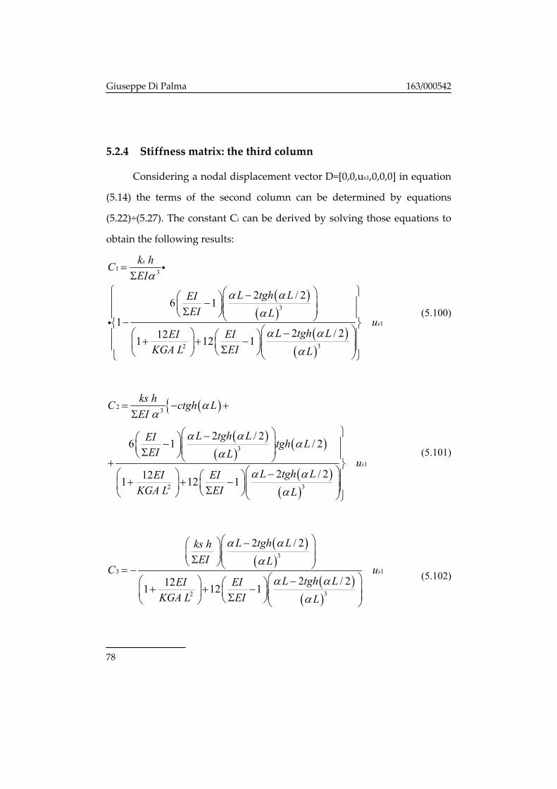
5.Stiffness matrix 55 5.1Identification of the problem 55 5.2Coefficients of the stiffness matrix 57
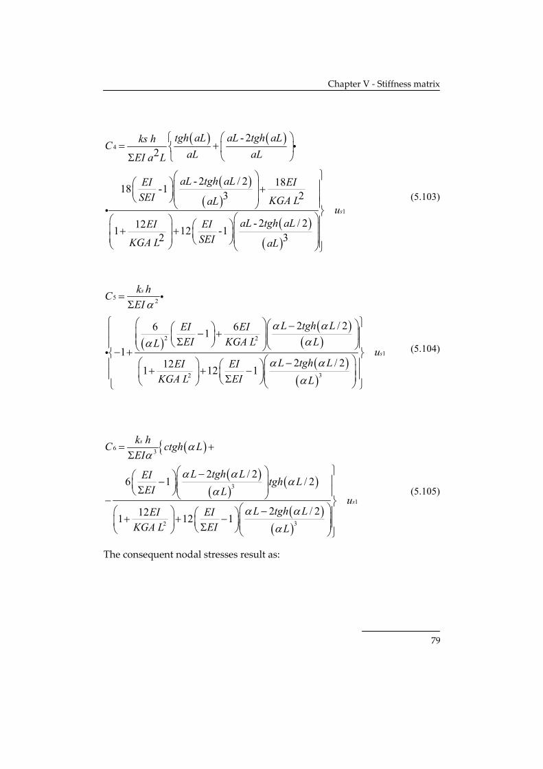
5.2.1 General procedure for deriving the integration constants 57 5.2.2 Stiffness matrix: the first column 62 5.2.3 Stiffness matrix: the second column 69 5.2.4 Stiffness matrix: the third column 78 5.2.5 Completing the stiffness matrix 90
5.3Vector of the external nodal force and vector nodal forces equivalent to distributed action 91
5.3.1 Vector of the external nodal forces 91 5.3.2 Vector nodal forces equivalent to distributed actions. 91
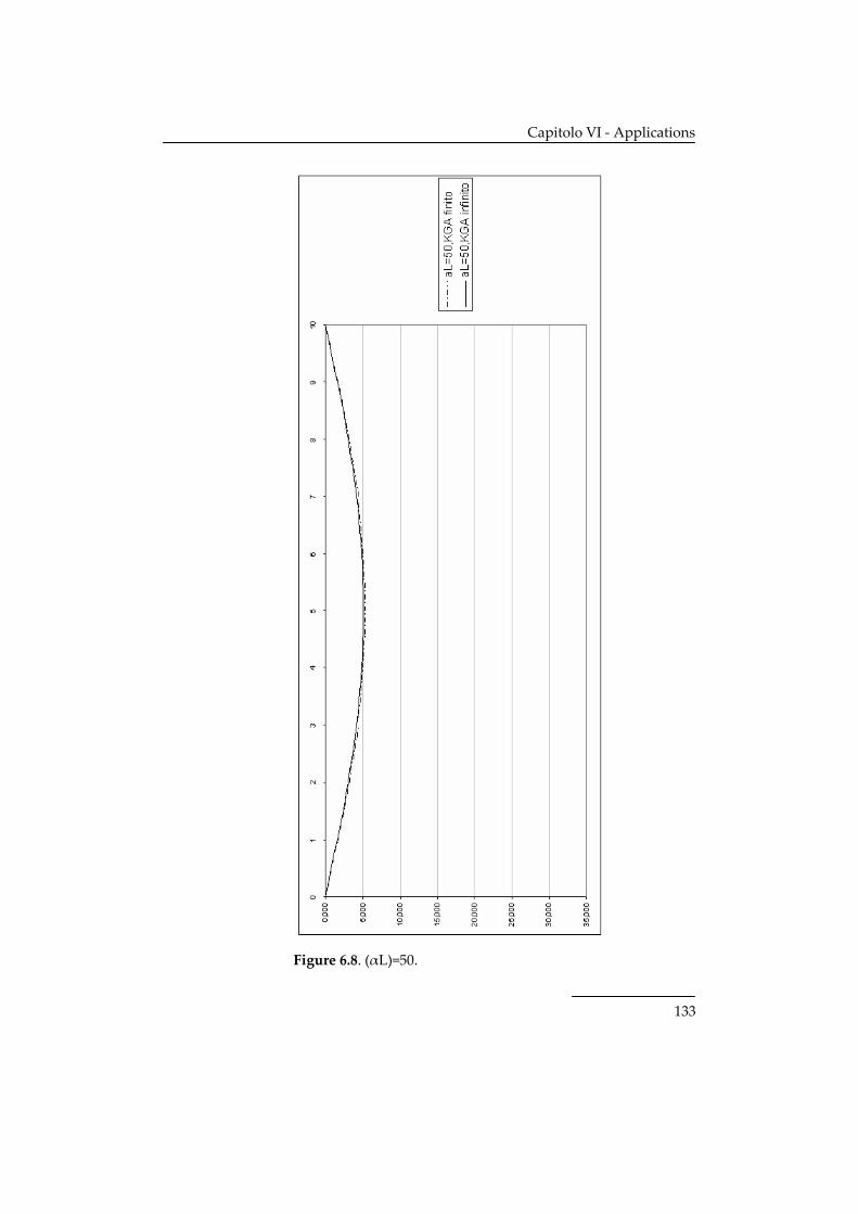
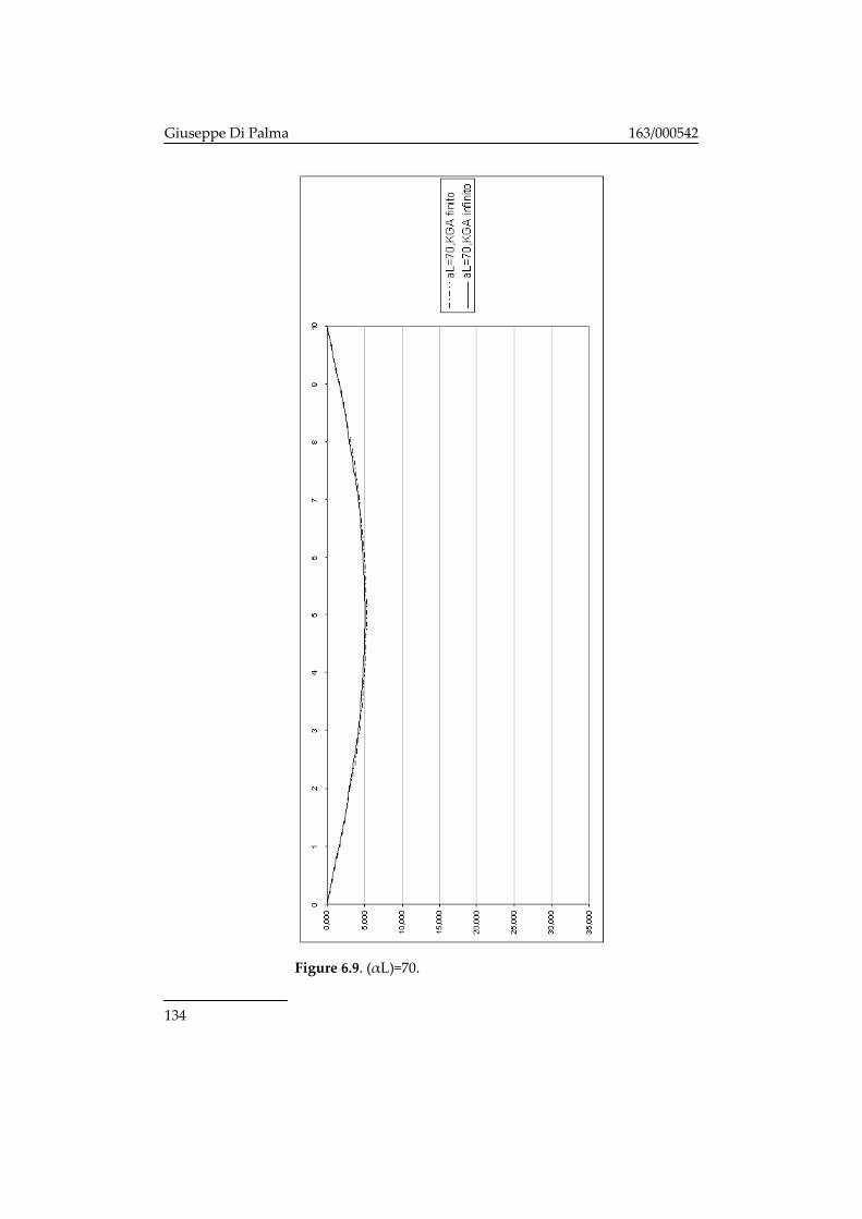
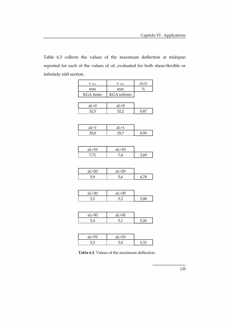
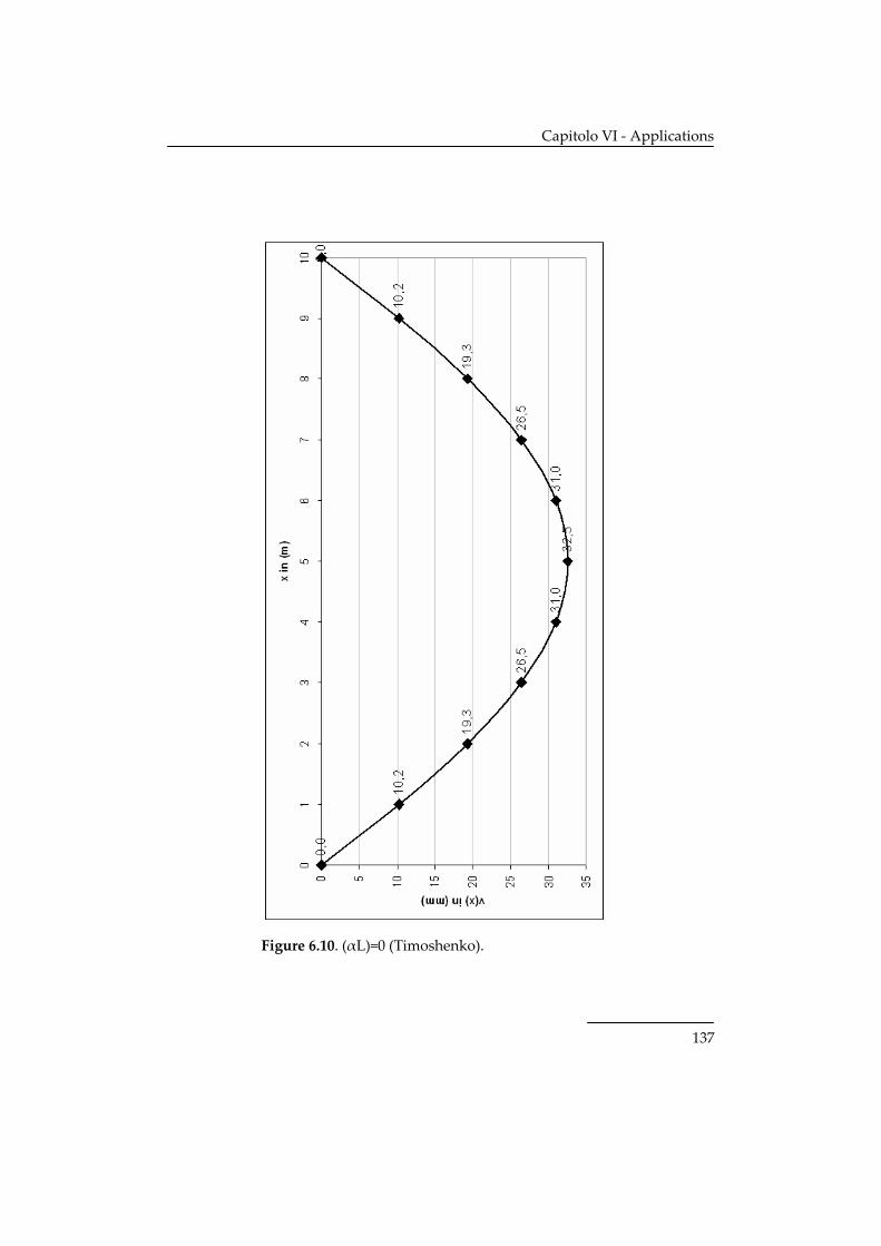
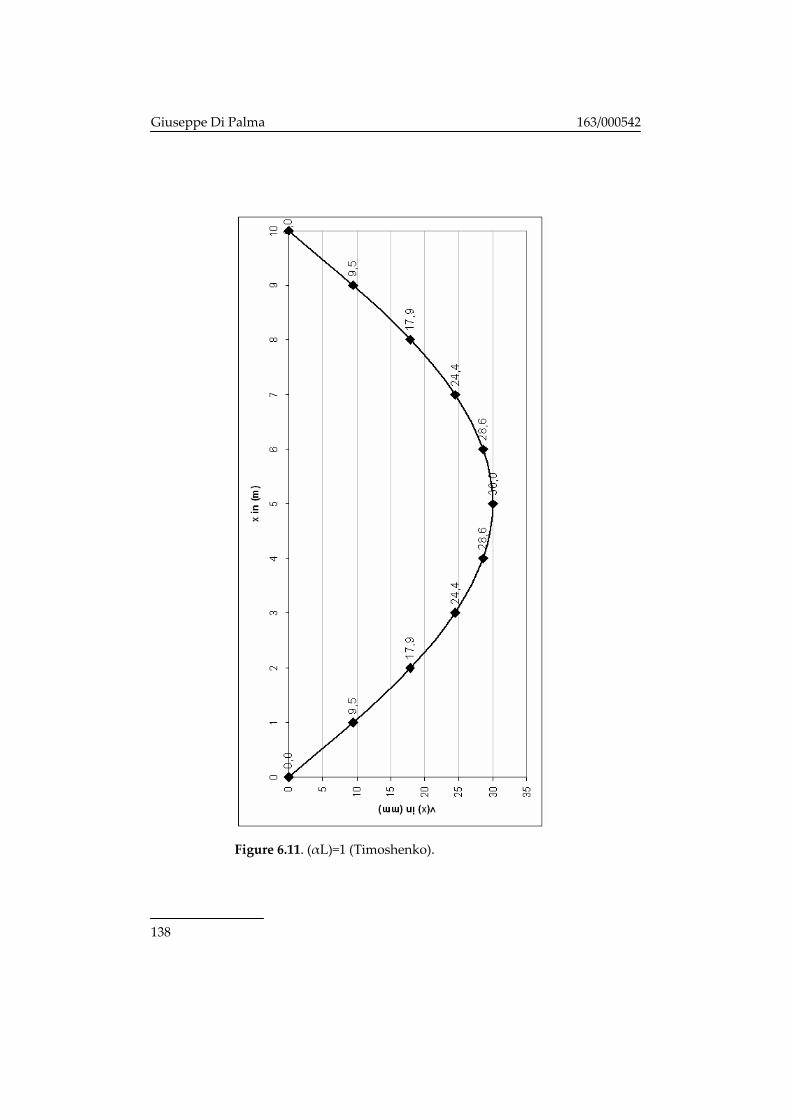
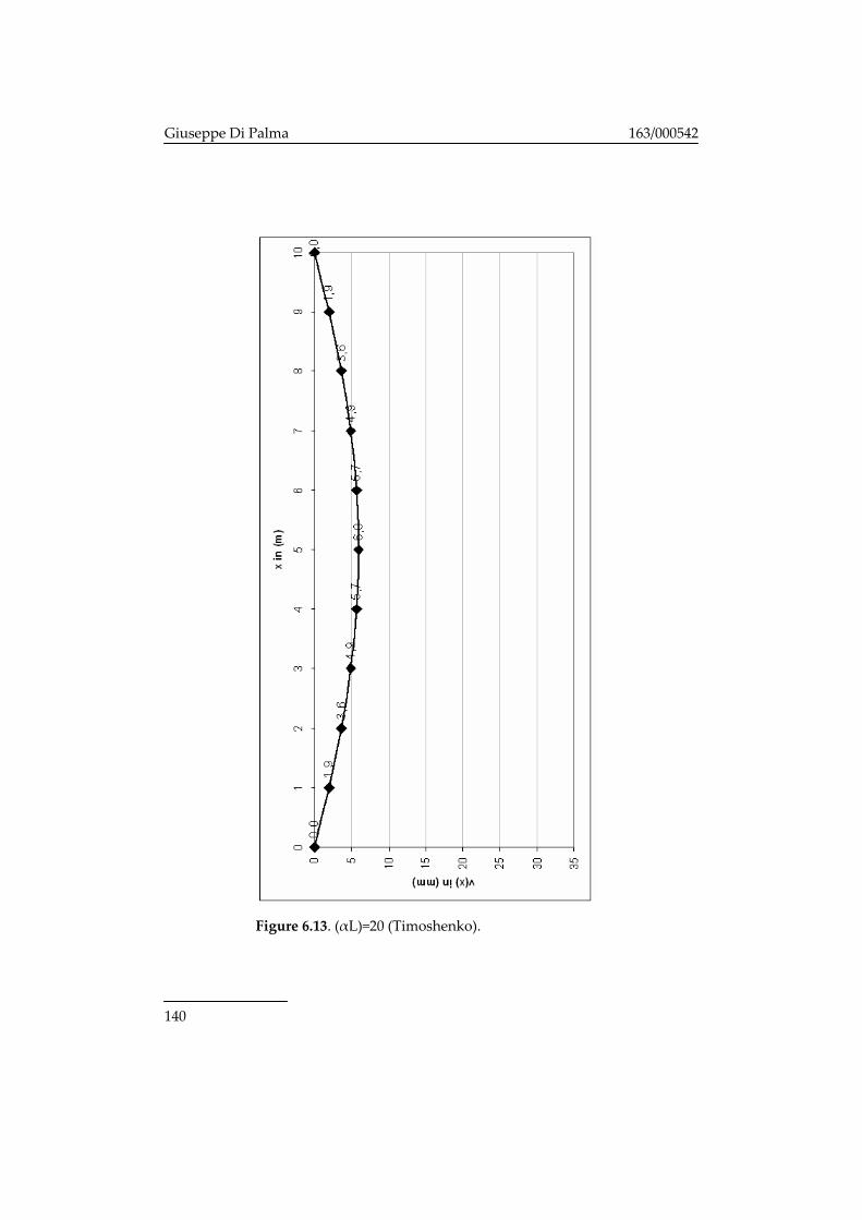
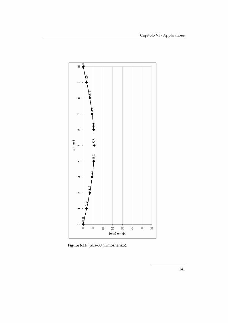
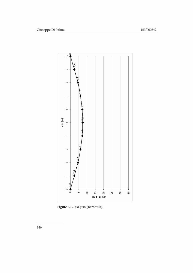
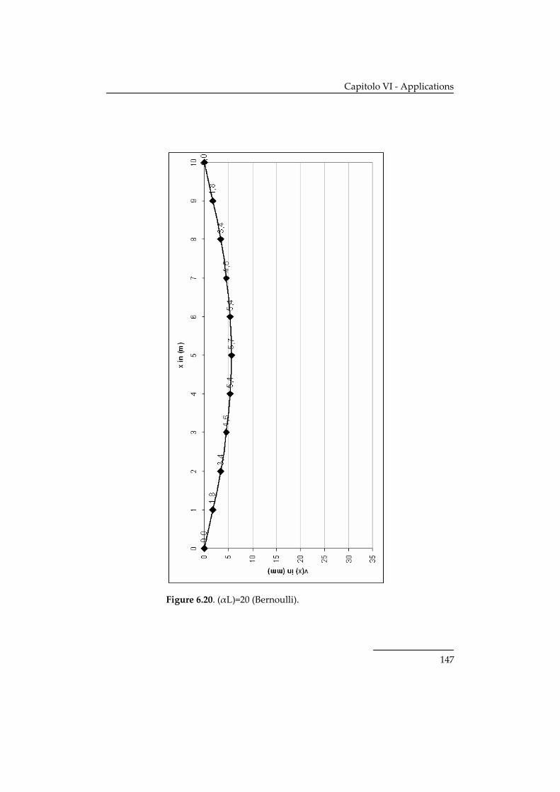
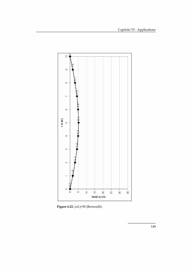
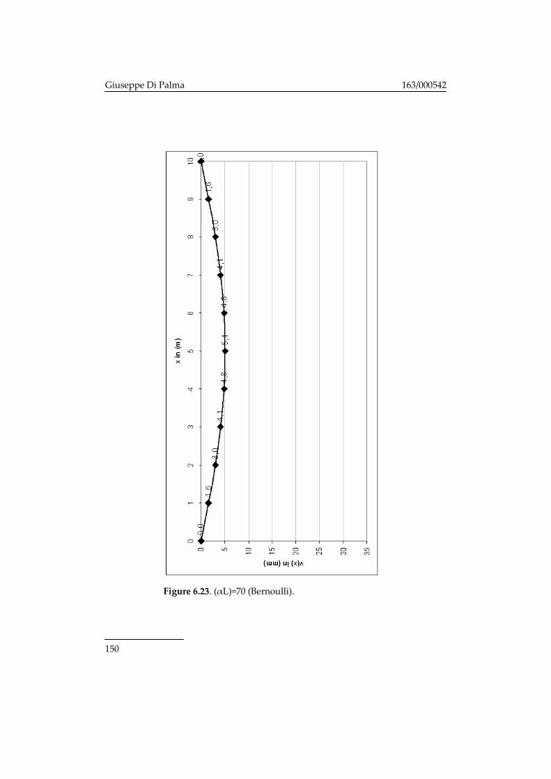
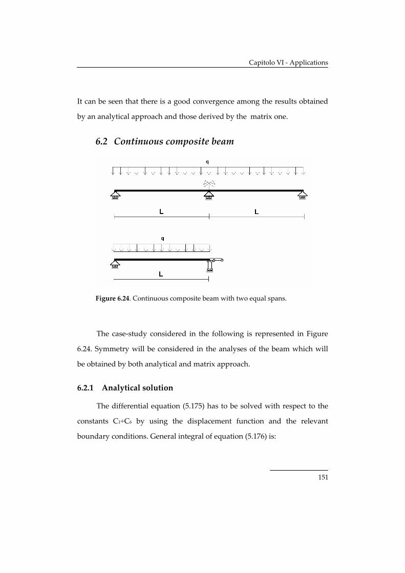
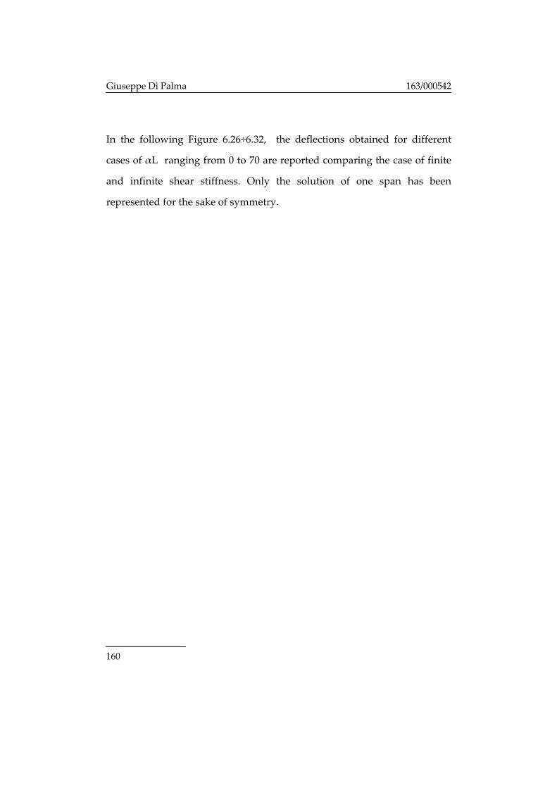
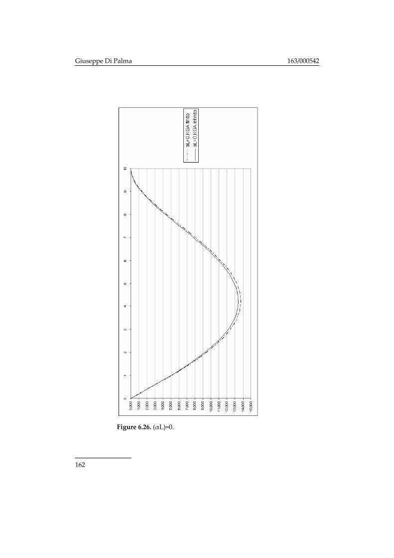
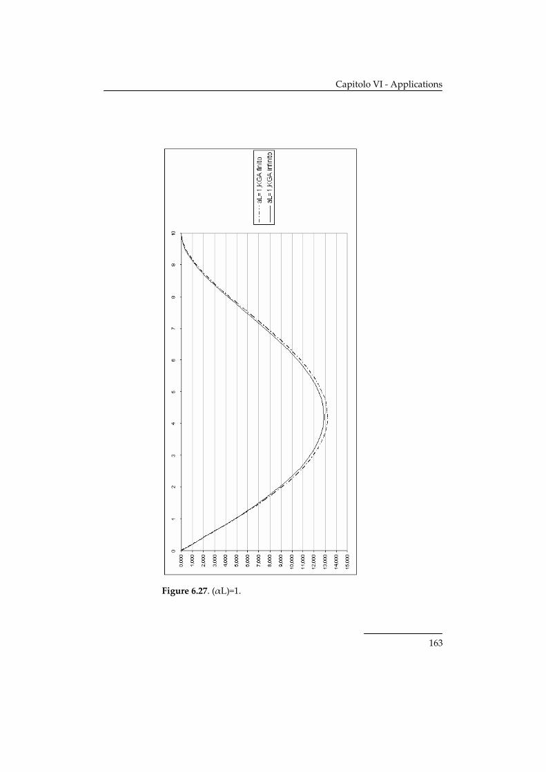
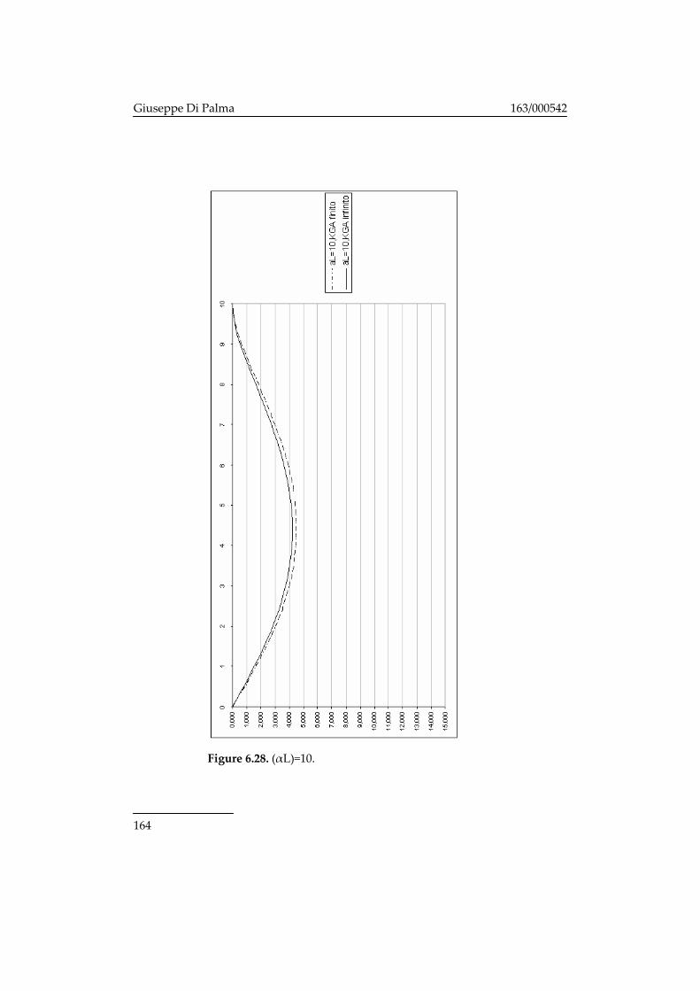
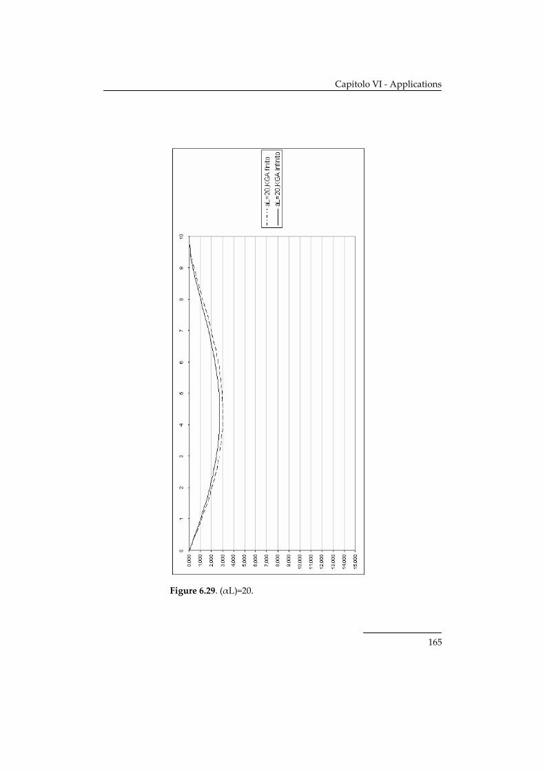
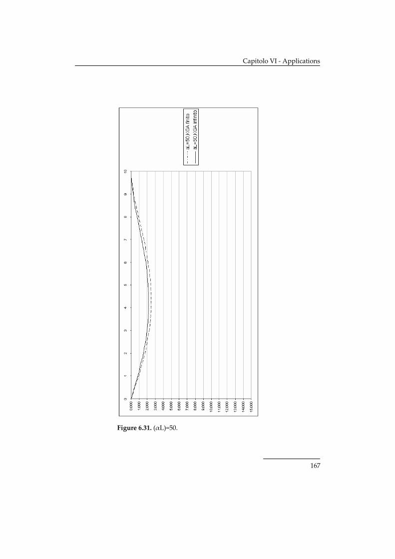
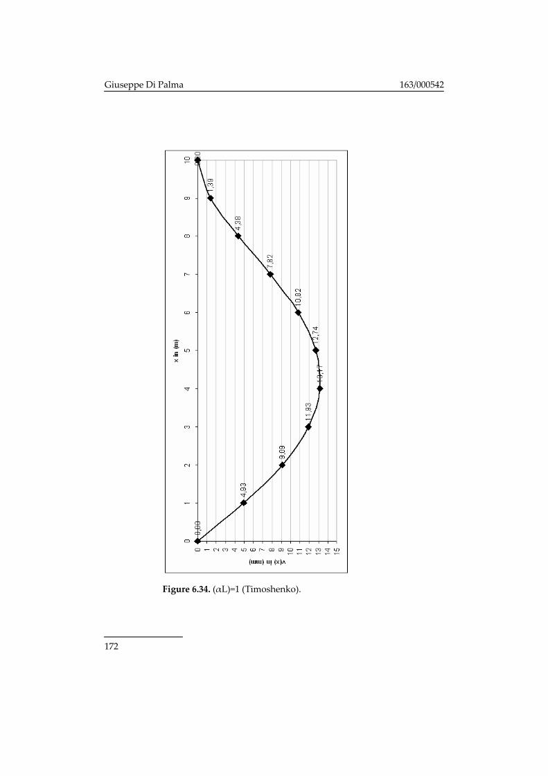
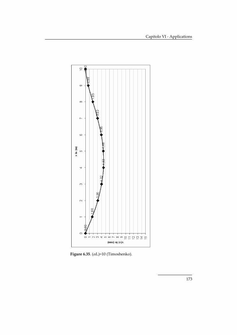
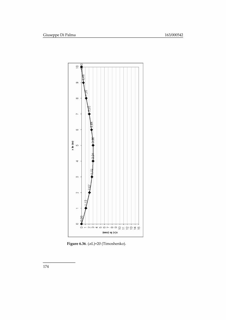
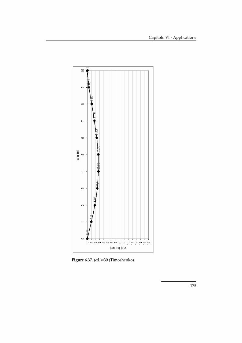
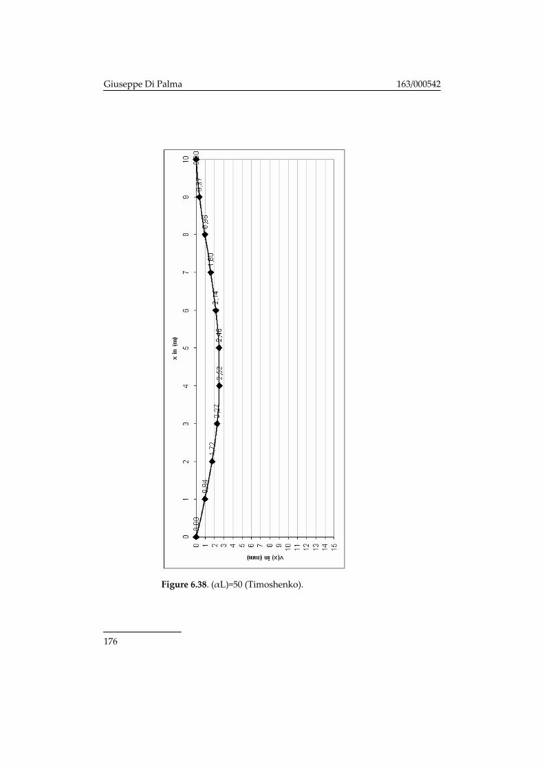
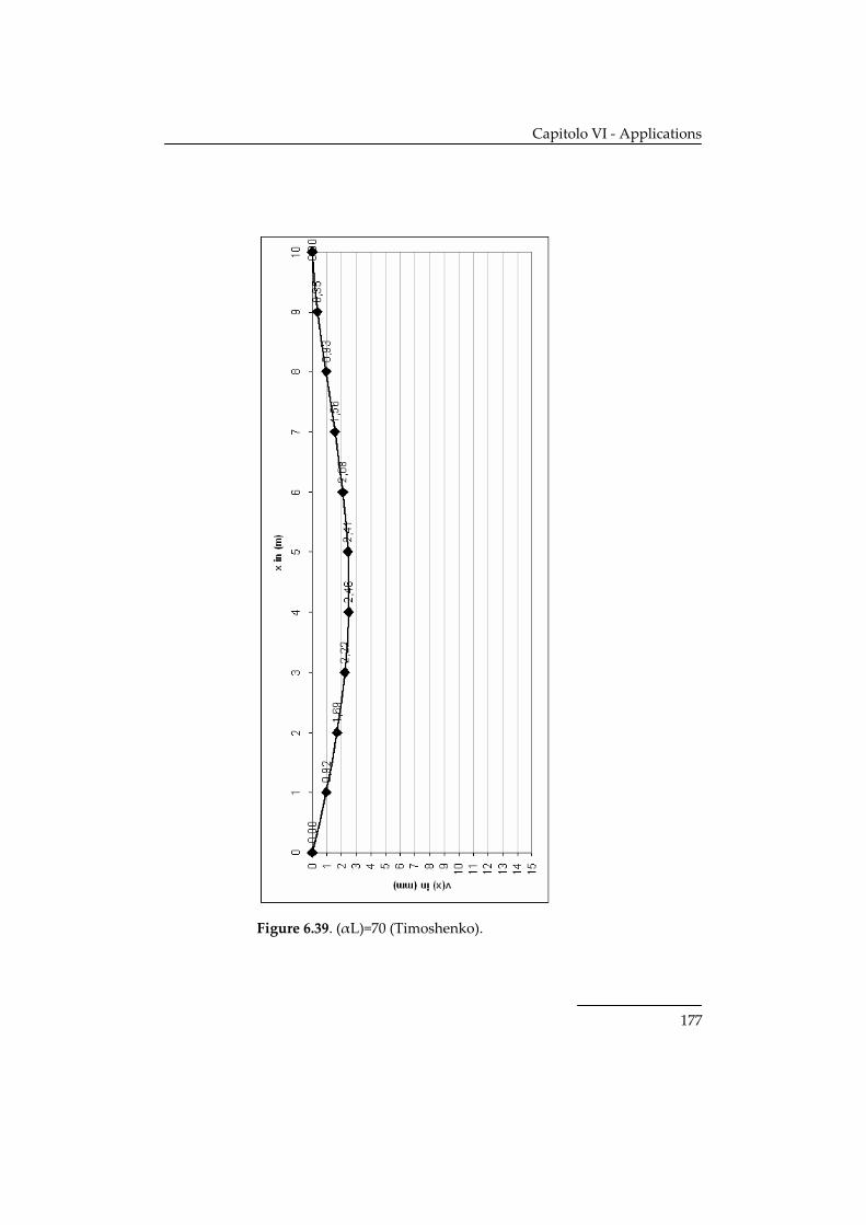
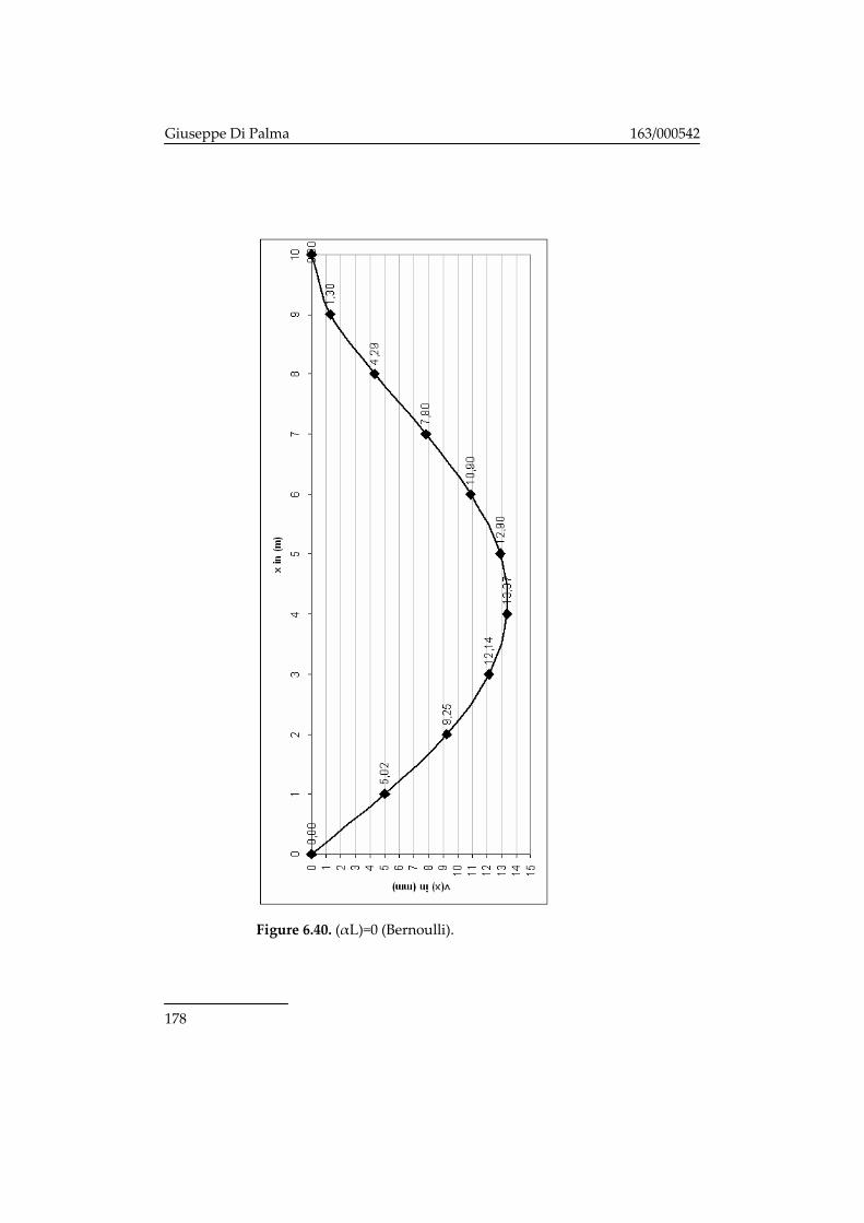
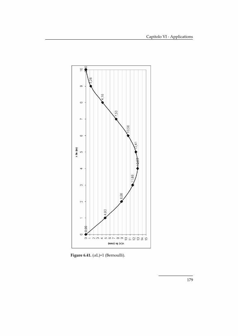
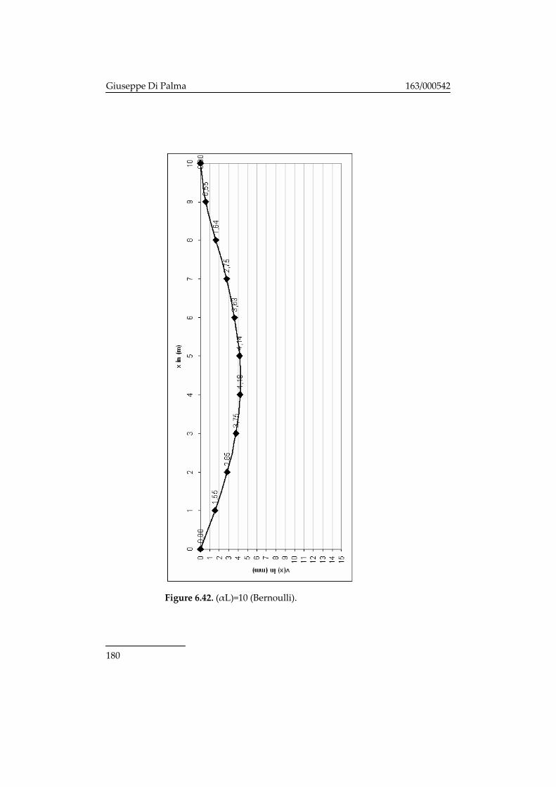
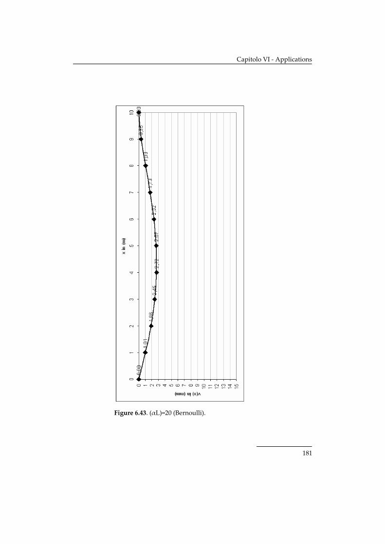
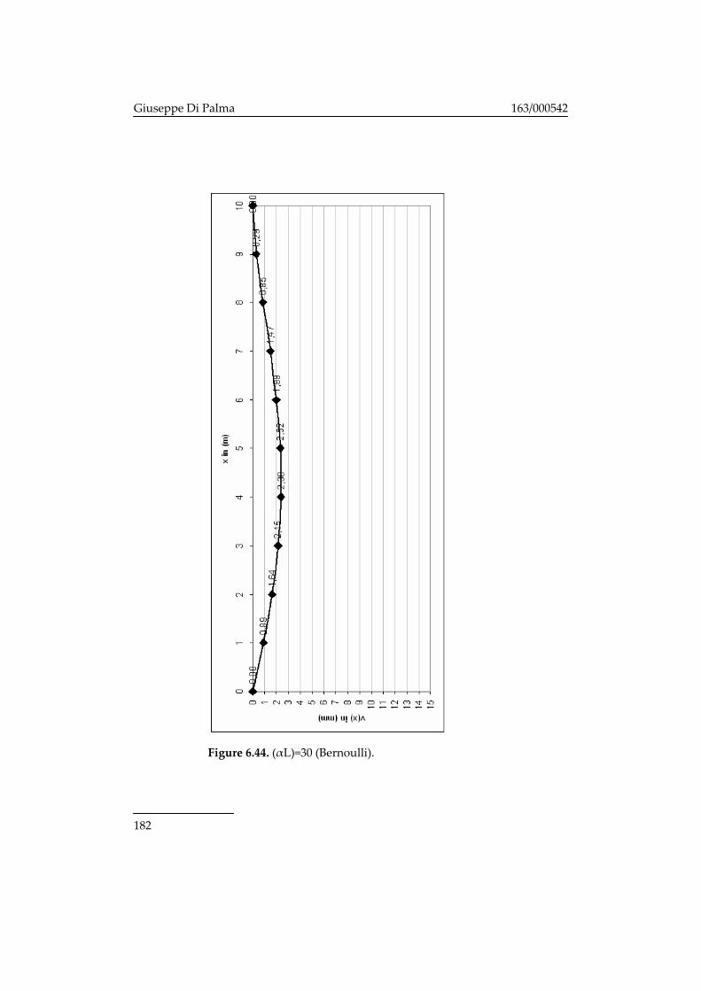
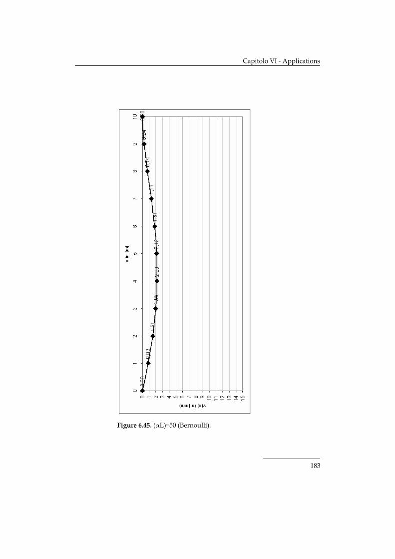
6.Applications 117 6.1Simply‐supported composite beam 117
6.1.1 Solutions in terms of displacements 120 6.1.2 Comparisons between Timoshenko and Bernoulli model 123 6.1.3 Solution by matrix method 136
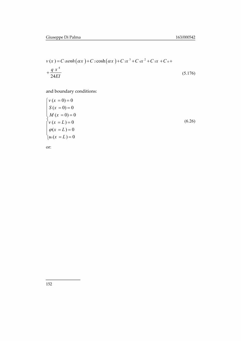
6.2Continuous composite beam 151 6.2.1 Analytical solution 151 6.2.2 Comparison between Timoshenko and Bernoulli model 158 6.2.3 Solution by matrix method 170 6.2.4 Solutions in terms of forces 185 6.2.5 Comparisons between Timoshenko model and Bernoulli model 186
7.Conclusions 198
8.Bibliography 199
Page 8
1
1. Introduction
Structural behaviour of steel‐concrete composite beams and
structures is generally influenced by several phenomena related to the
behaviour of steel and concrete as well as the behaviour of shear
connectors.
The present thesis is aimed to derive stiffness matrix of the composite beam
under sufficiently general hypotheses. In particular, after a through
examination of previous works in the scientific literature, various
contributions can be found, and a complete analytical derivation of the
stiffness matrix for composite beams in partial interaction behaving to
Bernoulli theory, has been already formulated, starting from the original
Newmark theory.
1.1 State of the art
Timoshenko [1] developed a theory for composite beams with two
bonded materials using Bernoulli‐Euler beam theory for each component
and constraining transverse displacements to be equal. Newmark et al. [2]
established the governing equations for elastically connected steel‐concrete
beams neglecting uplift and friction. Adekola [3] extended this work by
including uplift and frictional effects. He proposed a finite‐
Page 9
Giuseppe Di Palma 163/000542
2
difference procedure for solving the differential equation for uplift and
axial forces. Robinsion and Naraine [4] addressed the issue of whether the
forces at the interface act on the concrete slab or pull on the steel beam.
Cosenza and Mazzolani [5] proposed a new solution procedure that is
suitable for general loading conditions and McGarraugh and Baldwin [6]
used a simple analytical model to prove that the strength of a composite
girder with partial interaction can be derived by nonlinear interpolation of
the beam strength for the extreme cases of no interaction and full
interaction. For the study of the nonlinear behavior of composite members
the existing studies can be grouped into the following two categories: (1)
Finite‐element models utilizing beam, plate, shell, or brick finite elements
to represent in great detail the constituents of the composite structural
element (such models are rather complex, very computationally intensive,
and limited to monotonic loads); and (2) 1D beam elements that capture
salient features of the nonlinear behavior of composite girders within the
framework of Navier‐Bernoulli beam theory. Within the latter category
proposed models can be grouped into three categories: (1) Full composite
action models based on displacement interpolation functions with fiber
discretization of the cross section and uniaxial stress‐strain relations of the
constituent materials, as proposed by Mirza and Skrabek [7] for the
analysis of composite columns under uniaxial bending and El‐Tawil et al.
[8] under biaxial bending; (2) models of the partial composite action
between concrete and steel based on displacement interpolation functions
for the concrete and steel component of the composite element, which
Page 10
Chapter I ‐ Introduction
3
readily supply the relative longitudinal or transverse displacement at the
interface; in this category belong the study by Daniel and Crisinel [9] for
composite beams under monotonic loads, the study by Amadio and
Fragiacomo [10] for the effect of concrete creep and shrinkage in composite
beams, the study by Hajjar et al. [11] for concrete‐ filled, steel tube columns,
and the study by Salari et al. [12] for composite beams under cyclic loads;
and (3) recent models that attempt to overcome the limitations of
displacement‐based models by the use of force interpolation functions
(flexibility formulation); interest in this type of nonlinear model increased
after the work by Ciampi and Carlesimo [14], who are the first to propose a
consistent implementation of the flexibility formulation of a nonlinear
Bernoulli beam element within the framework of a general purpose
nonlinear analysis program. The selection of suitable force interpolation
functions that strictly satisfy element equilibrium is rather straightforward
for the case of a nonlinear Bernoulli beam element; in this case the fiber
discretization of the cross section affords a convenient means of describing
the complex hysteretic response of members under cyclic loading histories
(Spacone et al. [15]). Difficulties arise, however, in the selection of force
interpolation functions that strictly satisfy equilibrium for cases that
involve interaction between beam displacements and internal forces.
Examples are an anchored reinforcing bar, a prestressed concrete girder, a
steel‐concrete girder with partial composite action, and a slender column.
Attempts to extend the advantages of a force‐based flexibility formulation
to these cases have been recently reported (Yassin [16]; Ayoub and Filippou
Page 11
Giuseppe Di Palma 163/000542
4
[17]; Monti et al. [19]; Neuenhofer and Filippou [20]; Salari et al.). With the
exception of the study by Neuenhofer and Filippou, which is, however,
limited to linear elastic material behavior, the other studies resort to ad hoc
assumptions for overcoming the difficulty of deriving force interpolation
functions that strictly satisfy equilibrium. The formulations by Yassin,
Monti et al., and Ayoub and Filippou limit the interaction between the two
components to the end nodes of the element and assume a linear
interpolation of bond or friction forces in between. This requires a small
element size for accurate local response eliminating one of the advantages
of the flexibility‐based formulation (Neuenhofer and Filippou). To
overcome this weakness Salari et al. introduced higher order bond force
distribution functions. The formulation, however, lacks clarity about the
relation between the slip distribution in the element and the element end
displacements. Analytical results reveal interelement discontinuities of slip
displacements in violation of variational principles. It is also not clear that
the element can be extended to accommodate distributed element loads. In
view of the limitations of the displacement formulation (Neuenhofer and
Filippou) and the difficulty of selecting force interpolation functions that
strictly satisfy equilibrium for problems with strong interaction between
displacements and internal forces, Ayoub and Filippou recently proposed a
consistent mixed formulation of the anchored reinforcing bar problem with
independent interpolation functions for the axial displacements and the
reinforcing steel stresses. This formulation combines the advantages of the
Page 12
Chapter I ‐ Introduction
5
displacement and force formulations while overcoming most of their
limitations.
More recently, Wu and Xu [22],[24] considered the Timoshenko kinematics
for both the connected members in order to derive a more general model
under similar hypotheses. Three applications were proposed in the
mentioned papers:
• simulation of the behaviour of a beam in bending considering shear
flexibility;
• buckling analysis of the axially loaded beam‐columns taking into
account second order effects due to flexural deflection;
• dynamics and vibration analysis of composite beams.
The authors provided some examples and the deflection values at the
midspan for all the previously mentioned three cases. The value of the
Euler critical load has been also provided regarding the buckling of the
beam. This work is the starting point of the present thesis whose final result
consists in deriving the close‐form expression for the stiffness matrix,
including the shear flexibility effects .
Ranzi and Zona [23] worked at the same problem, including the shrinkage
effects using the Volterra equation and they solved it by approximating
with a linear function.
A recent research by Sakr and Sakla [26] deals with beams with incomplete
connections, in presence of cracking. The distributed effects are taken into
account both in the cracked and uncracked stage. The non‐linear behaviour
of the connection is modelled according to Ollgard as usually
Page 13
Giuseppe Di Palma 163/000542
6
accepted also within the previously mentioned papers. The stress strain
relationship is the Volterra one which includes a stress function at a generic
instant, so that it can be only numerically solved step by step. As far as the
stress‐strain relationship of steel, two Young moduli have to be used: one
for the steel beam and one for the internal reinforcement of the concrete
slab. It can be seen that the setting of this method is just the same of the
FEM analysis. It has been observed a substantial influence of the long‐term
deformability of connection, especially for simply supported beams.
Finally, more advanced studies try to model the stress‐strain relationship of
the materials with non‐linear functions and take into account the
distributed effects of the cracking.
The present work frames itself into the linear analysis of composite beams
with flexible connection, and its purposes are to give a further contribution
about shear strains and stresses.
Page 14
7
2. A Timoshenko‐based model for composite
beams in partial interaction
The key features of a brand‐new model for simulating the behaviour
of steel‐concrete composite beams in partial interaction, looking after the
shear flexibility of both concrete slab and steel beam will be proposed.
2.1 Key geometric and mechanical properties of the
composite cross section
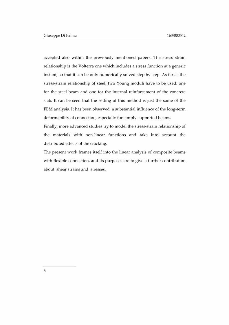
The typical cross section of a steal concrete composite beam is
represented in the Figure 2.1.
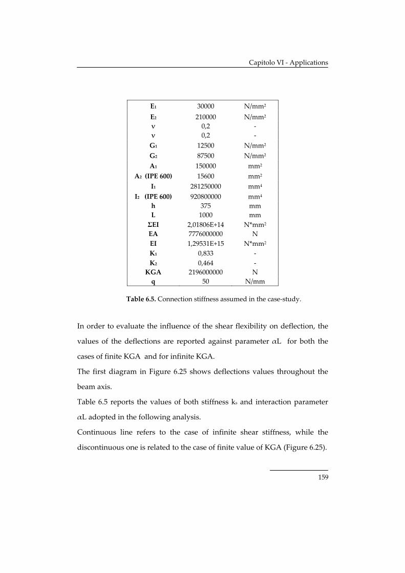
Figure 2.1. Properties of the cross section.
Page 15
Giuseppe Di Palma 163/000542
8
A geometric centroid of the section as a whole can be easily defined and its
position can be referred to the centroids of steel beam and concrete slab
through the following equations:
2 2 1 11 1 1 2 2 2 1 2
1 1 2 2 1 1 2 2,E A E AE A y E A y y h y h
E A E A E A E A= ⇒ = =
+ + (2.1)
2.2 Model equations
The general equations of the mentioned model will be formulated in
the present section.
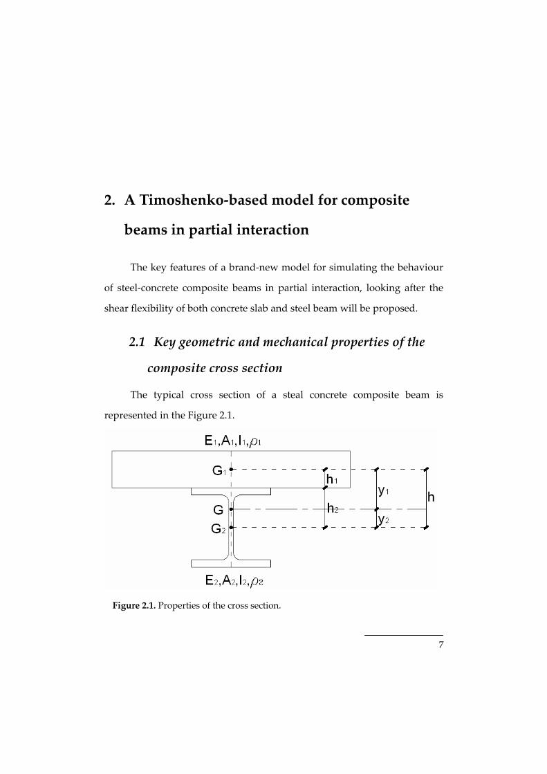
2.2.1 Equilibrium equations
The governing differential equations will be derived considering the
external actions and the internal (generalized) stresses represented in
Figure 2.2 .
Figure 2.2. An infinitesimal element of the composite beam.
Page 16
Chapter II –A Timoshenko‐based model for composite beams in partial interaction
9
Among the former ones, the inertial actions can be defined as follows:
,
,
d tt
d tt
F AvM I
ρρ ϕ
= −= −
(2.2)
where:
1 1 2 2
1 1 2 2
A A AI I I
ρ ρ ρρ ρ ρ
= += +
(2.3)
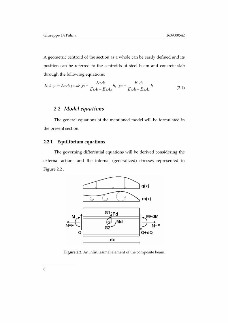
Second order effects are also considered in this stage. Figure 2.3 shows that
the axial force in Timoshenko beam is directed as the axis of the beam
therefore it is not orthogonal to the cross section because of the shear
flexibility (see the equation (2..4)):
, xvγ ϕ= + (2.4) As a result, the angle between the axial direction and the horizontal one is
defined through the function v(x); according to Figure 2.3 the second
derivative of deflection v(x) is always non‐positive (the x‐ axe is positive
towards the right and the deflection is positive towards the bottom)
therefore the second derivative is negative.
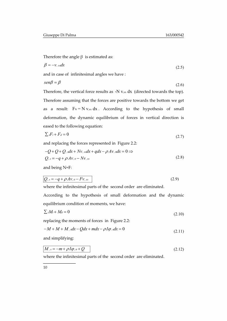
Figure 2.3. Calculation of the force FN.
Page 17
Giuseppe Di Palma 163/000542
10
Therefore the angle β is estimated as:
, xxv dxβ = − (2.5)
and in case of infinitesimal angles we have :
senβ β= (2.6) Therefore, the vertical force results as ,xx-N v dx (directed towards the top).
Therefore assuming that the forces are positive towards the bottom we get
as a result: N ,xxF = N v dx . According to the hypothesis of small
deformation, the dynamic equilibrium of forces in vertical direction is
eased to the following equation:
0i i dF F∑ + = (2.7) and replacing the forces represented in Figure 2.2:
, , ,
, , ,
0x xx tt
x tt xx
Q Q Q dx Nv dx qdx Av dxQ q Av Nv
ρρ
− + + + + − = ⇒= − + −
(2.8)
and being N=F:
, , ,x tt xxQ q Av Fvρ= − + − (2.9)
where the infinitesimal parts of the second order are eliminated.
According to the hypothesis of small deformation and the dynamic
equilibrium condition of moments, we have:
0i i dM M∑ + = (2.10) replacing the moments of forces in Figure 2.2:
,, 0ttxM M M dx Qdx mdx I dxρ ϕ− + + − + − = (2.11)
and simplifying:
, ,x ttM m I Qρ ϕ= − + + (2.12)
where the infinitesimal parts of the second order are eliminated.
Page 18
Chapter II –A Timoshenko‐based model for composite beams in partial interaction
11
2.2.2 Constitutive laws
General constitutive (stress‐strain) relationships have to be
introduced to formulate the composite beam model.
Anelastic deformation can be also considered in those relationships for the
sake of generality.
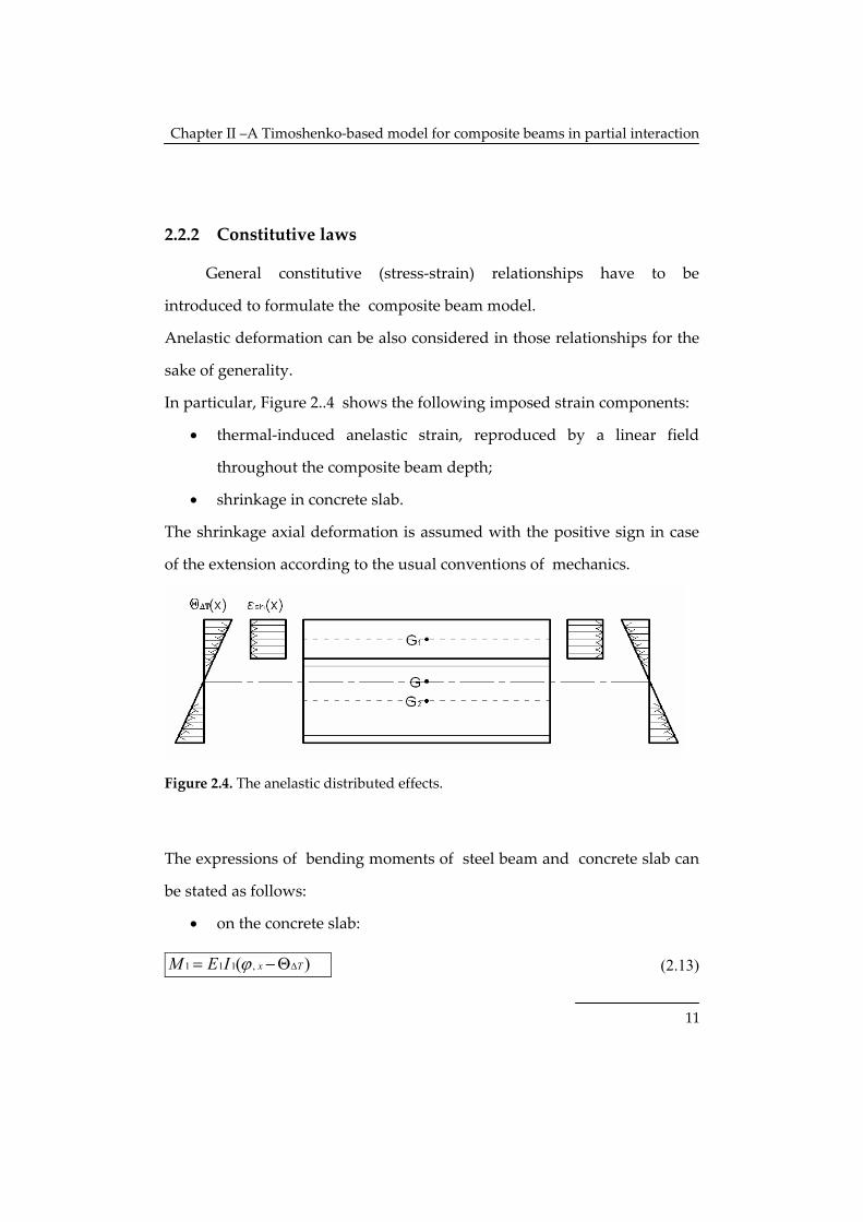
In particular, Figure 2..4 shows the following imposed strain components:
• thermal‐induced anelastic strain, reproduced by a linear field
throughout the composite beam depth;
• shrinkage in concrete slab.
The shrinkage axial deformation is assumed with the positive sign in case
of the extension according to the usual conventions of mechanics.
Figure 2.4. The anelastic distributed effects.
The expressions of bending moments of steel beam and concrete slab can
be stated as follows:
• on the concrete slab:
1 1 1 ,( )x TM E I ϕ ∆= −Θ (2.13)
Page 19
Giuseppe Di Palma 163/000542
12
• on the steel beam:
2 2 2 ,( )x TM E I ϕ ∆= −Θ (2.14)
Considering the (generalized) stress‐strain relationship for shear, the
following formula can be introduced.
,( )xQ KGA v ϕ= + (2.15)
As a basic feature of the present model, shear force and the corresponding
(generalized) strain are not defined for either the steel beam or the concrete
slab, but deal with the composite cross section as a whole; the shear
stiffness of the beam section is defined as follows:
1 1 1 2 2 2KGA K G A K G A= + (2.16) For the sake of simplicity, the following assumption will be considered for
bending stiffness and other parameters:
1 1 2 2
1 1 2 2 2
1 1 2 2
2 21 1 2 2 1 1 2 2
1 1 2 2 1 1 2 2
21 1 2 22
1 1 2 2
1 1 2 2
1 1 2 2
s
s s
s
EI E I E IE A E AEI EI hE A E A
EI k E A E A h E A E A EI EAk E A E A EI E A E A k
E A E A hkE A E A EI
E A E AEAE A E A
α
α
Σ = +
= Σ + =+
⎛ ⎞Σ + Σ= + =⎜ ⎟Σ +⎝ ⎠
⎛ ⎞+= +⎜ ⎟Σ⎝ ⎠
=+
(2.17)
Page 20
Chapter II –A Timoshenko‐based model for composite beams in partial interaction
13
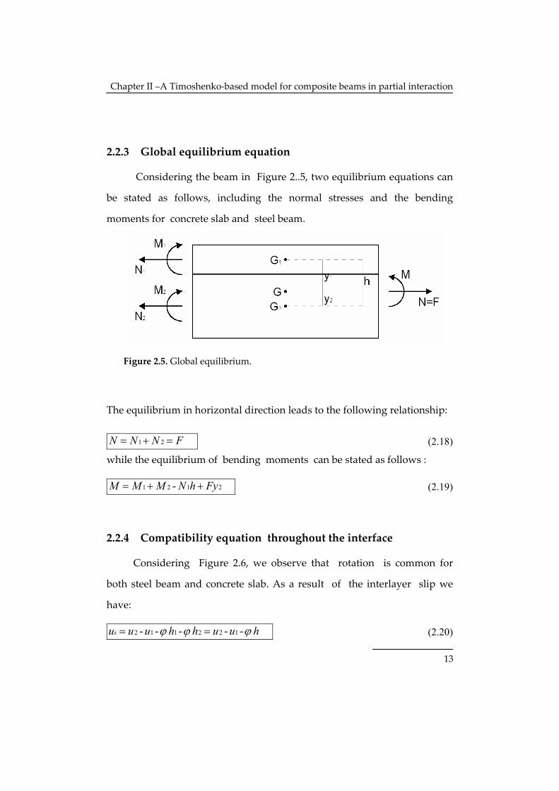
2.2.3 Global equilibrium equation
Considering the beam in Figure 2..5, two equilibrium equations can
be stated as follows, including the normal stresses and the bending
moments for concrete slab and steel beam.
Figure 2.5. Global equilibrium.
The equilibrium in horizontal direction leads to the following relationship:
1 2N N N F= + = (2.18)
while the equilibrium of bending moments can be stated as follows :
1 2 1 2-M M M N h Fy= + + (2.19)
2.2.4 Compatibility equation throughout the interface
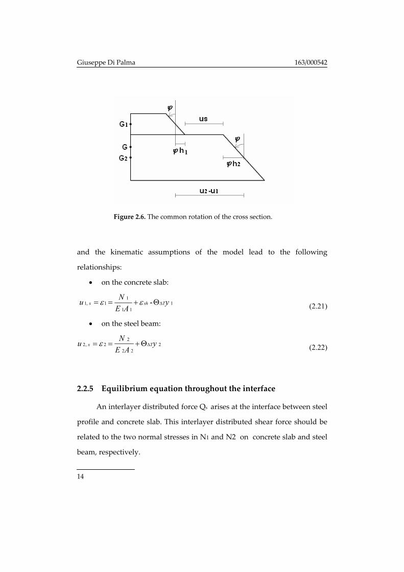
Considering Figure 2.6, we observe that rotation is common for
both steel beam and concrete slab. As a result of the interlayer slip we
have:
2 1 1 2 2 1- - - - -su u u h h u u hϕ ϕ ϕ= = (2.20)
Page 21
Giuseppe Di Palma 163/000542
14
Figure 2.6. The common rotation of the cross section.
and the kinematic assumptions of the model lead to the following
relationships:
• on the concrete slab:
1
1, 1 11 1
-x sh TNu yE A
ε ε ∆= = + Θ (2.21)
• on the steel beam:
22, 2 2
2 2x T
Nu yE A
ε ∆= = +Θ (2.22)
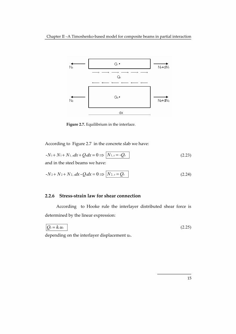
2.2.5 Equilibrium equation throughout the interface
An interlayer distributed force Qs arises at the interface between steel
profile and concrete slab. This interlayer distributed shear force should be
related to the two normal stresses in N1 and N2 on concrete slab and steel
beam, respectively.
Page 22
Chapter II –A Timoshenko‐based model for composite beams in partial interaction
15
Figure 2.7. Equilibrium in the interface.
According to Figure 2.7 in the concrete slab we have:
1 1 1,- 0x sN N N dx Q dx+ + + = ⇒ 1, -x sN Q= (2.23)
and in the steel beams we have:
2 2 2,- - 0x sN N N dx Q dx+ + = ⇒ 2, x sN Q= (2.24)
2.2.6 Stress‐strain law for shear connection
According to Hooke rule the interlayer distributed shear force is
determined by the linear expression:
s s sQ k u= (2.25)
depending on the interlayer displacement us.
Page 23
16
3. Outline of the governing equations
The equations derived in the previous section can be condensed and
simplified to obtain the key set of simultaneous equations describing the
behaviour of shear flexible composite beams in partial interaction.
3.1 The system of three equations in three unknown
functions
Deriving the expression of the slip (2.20) and introducing the
definitions of normal strains (2.21)‐(2.22) we have:
, 1, 2, 2 1 , 2
2 2
1 1 11 , 2
1 1 2 2 1 1
1 , 12 2 1 1 2 2
,
-
1 1
s x xxs x x T
s s
sh T x T
sh T x
sh T x
Q N Nu h yk k E A
N F N Ny h yE A E A E A
Fy h NE A E A E A
h h
ε ε ϕ
ε ϕ
ε ϕ
ε ϕ
∆
∆ ∆
+ ∆
+ ∆
= = − = − − = +Θ +
−⎛ ⎞− + Θ − = +Θ − +⎜ ⎟⎝ ⎠
⎛ ⎞− Θ − = − + +⎜ ⎟⎝ ⎠
− Θ −
(3.1)
from which we get:
1, 1 ,2 2 1 1 2 2
1 ,2 2 1 1 2 2
1 1
1 1
xx s sh T x
ss s sh s T s x
FN k N h hE A E A E A
F k N k k k h k hE A E A E A
ε ϕ
ε ϕ
+ ∆
− ∆
⎛ ⎞⎛ ⎞= − − + − Θ − =⎜ ⎟⎜ ⎟⎝ ⎠⎝ ⎠⎛ ⎞= − + + + Θ +⎜ ⎟⎝ ⎠
(3.2)
and as a result:
Page 24
Chapter III ‐ Outline of the governing equations
17
1
1, ,2 2
sxx s s sh s T s x
F k NN k k k h k hE A EA
ε ϕ− ∆= − + + Θ + (3.3)
Furthermore, introducing the expressions of bending moments (2.13) and
(2.14) into the equation (2.19) we obtain :
1 1 , 2 2 , 1 2( ) ( )x T x TM E I E I N h Fyϕ ϕ∆ ∆= −Θ + −Θ − + (3.4)
from which we have:
1 2
, x TM N h Fy
EIϕ ∆
+ −= +Θ
Σ (3.5)
introducing the equation (3.5) into (3.4) we get :
1 1 21,
2 2
1 1 2
2 2
sxx s s sh s T
ss T s s sh s
Fk N M N h FyN k k k hE A EA EI
Fk N M N h Fyk h k k k hE A EA EI
ε
ε
∆
∆
+ −⎛ ⎞= − + + + +Θ +⎜ ⎟Σ⎝ ⎠+ −
− Θ = − + + +Σ
(3.6)
and the following expression can be finally obtained after some
mathematical simplification:
2
21, 1
2 2
11 sxx s s s sh
h k hM hyN k N k F kEA EI EI E A EIε
⎛ ⎞ ⎛ ⎞− + = − + +⎜ ⎟ ⎜ ⎟Σ Σ Σ⎝ ⎠⎝ ⎠ (3.7)
The definitions (2.17) can be introduced obtaining the following equation:
221, 1
2 2
1sxx s s sh
k hM hyN N k F kEI E A EI
α ε⎛ ⎞− = − + +⎜ ⎟Σ Σ⎝ ⎠ (3.8)
Deriving (2.19) and introducing (2.12) the following equation can be
obtained:
, 1, 2, 1, ,x x x x ttM M M N h m I Qρ ϕ= + − = − + + (3.9)
that is:
Page 25
Giuseppe Di Palma 163/000542
18
1 1 , , 2 2 , , 1, ,
, , 1, ,
( ) ( )( )
xx T x xx T x x tt
xx T x x tt
E I E I N h m I QEI N h m I Q
ϕ ϕ ρ ϕϕ ρ ϕ
∆ ∆
∆
−Θ + −Θ − = − + +Σ −Θ − = − + +
(3.10)
and the following equation can be finally obtained:
, , , 1,xx T x tt xEI EI I N h m Qϕ ρ ϕ∆ −Σ −Σ Θ − + = (3.11)
Finally, deriving equation (2.15), through the (2 .9) one gets:
, , , , ,( )x xx x tt xxQ KGA v q Av Fvϕ ρ= + = − + − (3.12)
that is finally:
, , , ,( )xx x xx ttKGA v Fv Av qϕ ρ−+ + = − (3.13)
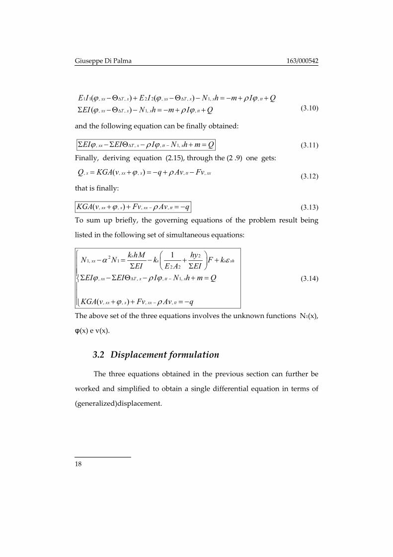
To sum up briefly, the governing equations of the problem result being
listed in the following set of simultaneous equations:
221, 1
2 2
, , , 1,
, , , ,
1
( )
sxx s s sh
xx T x tt x
xx x xx tt
k hM hyN N k F kEI E A EI
EI EI I N h m Q
KGA v Fv Av q
α ε
ϕ ρ ϕ
ϕ ρ
∆ −
−
⎧ ⎛ ⎞− = − + +⎜ ⎟⎪ Σ Σ⎝ ⎠⎪⎪Σ −Σ Θ − + =⎨⎪⎪
+ + = −⎪⎩
(3.14)
The above set of the three equations involves the unknown functions N1(x),
φ(x) e v(x).
3.2 Displacement formulation
The three equations obtained in the previous section can further be
worked and simplified to obtain a single differential equation in terms of
(generalized)displacement.
Page 26
Chapter III ‐ Outline of the governing equations
19
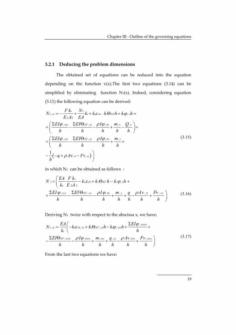
3.2.1 Deducing the problem dimensions
The obtained set of equations can be reduced into the equation
depending on the function v(x).The first two equations (3.14) can be
simplified by eliminating function N1(x). Indeed, considering equation
(3.11) the following equation can be derived:
( )
11, ,
2 2
, , , , ,
, , , ,
, ,1
sxx s s sh s T s x
xxx T xx ttx x x
xxx T xx ttx x
tt xx
F k NN k k k h k hE A EA
EI EI I m Qh h h h h
EI EI I mh h h h
q Av Fvh
ε ϕ
ϕ ρ ϕ
ϕ ρ ϕ
ρ
− ∆
∆
∆
= − + + Θ + =
⎛ Σ Σ Θ ⎞= − − + − =⎟⎜ ⎠⎝Σ Σ Θ⎛= − − + +⎜
⎝⎞− − + − ⎟⎠
(3.15)
in which N1 can be obtained as follows :
1 ,2 2
, , , , , ,
ss sh s T s x
s
xxx T xx ttx x tt xx
EA F kN k k h k hk E A
EI EI I m q Av Fvh h h h h h h
ε ϕ
ϕ ρ ϕ ρ
∆
∆
⎛= − + Θ − +⎜⎝
Σ Σ Θ ⎞+ − − + + − + ⎟⎠
(3.16)
Deriving N1 twice with respect to the abscissa x, we have:
,1, , , ,
, , , , , ,
xxxxxxx s sh xx s T xx s xxx
s
T xxxx ttxxx xxx xx ttxx xxxx
EA EIN k k h k hk h
EI I m q Av Fvh h h h h h
ϕε ϕ
ρ ϕ ρ
∆
∆
Σ⎛= − + Θ − + +⎜⎝
Σ Θ ⎞− − + + − + ⎟⎠
(3.17)
From the last two equations we have:
Page 27
Giuseppe Di Palma 163/000542
20
,, , ,
, , , , , ,
,2,
2 2
, , , , ,
xxxxxs sh xx s T xx s xxx
s
T xxxx ttxxx xxx xx ttxx xxxx
s xxxs sh s T s x
s
T xx ttx x tt xx
EA EIk k h k hk hEI I m q Av Fv
h h h h h hEA F k EIk k h k hk E A hEI I m q Av Fvh h h h h h
ϕε ϕ
ρ ϕ ρ
ϕα ε ϕ
ρ ϕ ρ
∆
∆
∆
∆
Σ⎛− + Θ − + +⎜⎝
Σ Θ ⎞− − + + − + +⎟⎠
Σ⎛− − + Θ − + +⎜⎝
Σ Θ ⎞− − + + − +
[
]
,2 2
, , , , ,,
, 22
2 2
1 0
s sx T s sh s T
s
xxx T xx ttx x tts x
xxs s sh
k h EA F kEI EI h k k hEI k E A
EI EI I m q Avk hh h h h h h
Fv hyFy k F kh E A EI
ϕ ε
ϕ ρ ϕ ρϕ
ε
∆ ∆
∆
+⎟⎠
⎛− Σ −Σ Θ − − + Θ +⎜Σ ⎝Σ Σ Θ
− + − − + + − +
⎞ ⎛ ⎞+ + + + − =⎟ ⎜ ⎟Σ⎠ ⎝ ⎠
(3.18)
The following equation can be obtained through suitable simplifications:
, , ,
2 2, ,
2, ,
2,
2
xxxxx ttxxx ttxxs s s
xxx ttxs s
tt xxxxs s
xxs
EI EA I EA AEAvhk hk hk
EI EA I EA I hEAhk hk EI
AEA AhEA F EAv vhk EI hk
F EA F hEAvhk EI
ρ ρϕ ϕ
ρ ρϕ α ϕ α
ρ ρα
α
α
⎛ ⎞ ⎛ ⎞ ⎛ ⎞Σ+ − + − +⎜ ⎟ ⎜ ⎟ ⎜ ⎟
⎝ ⎠ ⎝ ⎠ ⎝ ⎠⎛ ⎞ ⎛ ⎞Σ
+ − + − +⎜ ⎟ ⎜ ⎟Σ⎝ ⎠ ⎝ ⎠⎛ ⎞ ⎛ ⎞
+ − + +⎜ ⎟ ⎜ ⎟Σ⎝ ⎠ ⎝ ⎠⎛ ⎞
+ − + +⎜ ⎟Σ⎝ ⎠
−2
2 2 2 2 2 2
31 1 2 22
,
s s
s s sx
EA EAk h k FE A E A EI E A
E I k h E I k h k h EAhEAEI EI EI
α ϕ
⎛ ⎞− − +⎜ ⎟Σ⎝ ⎠
⎛ ⎞− − + + + =⎜ ⎟Σ Σ Σ ⎠⎝
Page 28
Chapter III ‐ Outline of the governing equations
21
( )
2 2
22
,
32 2
,
,
, ,
,
s s s
ssh s sh xx
s
sT s T xx
s
T xxxxs
EA hEA EA EA hEAq q xx m xhk EI hk hk EI
EA h EAkm xxx EA k EAhk EI
k h EA EI EAEAh k hEI hk
EA EIhk
α α
ε α ε
α α∆ ∆
∆
⎛ ⎞ ⎛ ⎞ ⎛ ⎞= − + − + − +⎜ ⎟ ⎜ ⎟ ⎜ ⎟Σ Σ⎝ ⎠ ⎝ ⎠ ⎝ ⎠
⎛ ⎞⎛ ⎞+ − − − − − − +⎜ ⎟⎜ ⎟ Σ⎝ ⎠ ⎝ ⎠
⎛ ⎞ ⎛ ⎞Σ+Θ − − +Θ − +⎜ ⎟ ⎜ ⎟Σ ⎝ ⎠⎠⎝
⎛ ⎞Σ+Θ ⎜ ⎟
⎝ ⎠
(3.19)
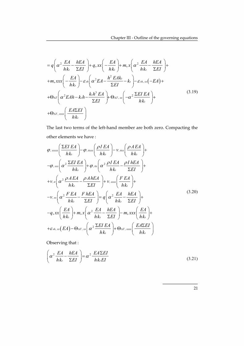
The last two terms of the left‐hand member are both zero. Compacting the
other elements we have :
, , ,
2 2, ,
2, ,
2 2,
xxxxx ttxxx ttxxs s s
xxx ttxs s
tt xxxxs s
xxs
EI EA I EA AEAvhk hk hk
EI EA I EA I hEAhk hk EI
AEA AhEA F EAv vhk EI hk
F EA F hEA EAv qhk EI hk
ρ ρϕ ϕ
ρ ρϕ α ϕ α
ρ ρα
α α
⎛ ⎞ ⎛ ⎞ ⎛ ⎞Σ− − +⎜ ⎟ ⎜ ⎟ ⎜ ⎟
⎝ ⎠ ⎝ ⎠ ⎝ ⎠⎛ ⎞ ⎛ ⎞Σ
− + − +⎜ ⎟ ⎜ ⎟Σ⎝ ⎠ ⎝ ⎠⎛ ⎞ ⎛ ⎞
+ − + +⎜ ⎟ ⎜ ⎟Σ⎝ ⎠ ⎝ ⎠⎛ ⎞
− − =⎜ ⎟Σ⎝ ⎠
( )
2
2, , ,
, , ,
s
s s s
sh xx T xx T xxxxs s
hEAEI
EA EA hEA EAq xx m x m xxxhk hk EI hk
EI EA EA EIEAhk hk
α
ε α∆ ∆
⎛ ⎞− +⎜ ⎟Σ⎝ ⎠
⎛ ⎞ ⎛ ⎞ ⎛ ⎞− + − − +⎜ ⎟ ⎜ ⎟ ⎜ ⎟Σ⎝ ⎠ ⎝ ⎠ ⎝ ⎠
⎛ ⎞ ⎛ ⎞Σ Σ+ −Θ +Θ⎜ ⎟ ⎜ ⎟
⎝ ⎠ ⎝ ⎠
(3.20)
Observing that :
2 2
s s
EA hEA EA EIhk EI hk EI
α α⎛ ⎞ Σ
− =⎜ ⎟Σ⎝ ⎠ (3.21)
Page 29
Giuseppe Di Palma 163/000542
22
and multiplying equation (3.20) by ks h/ ΣEI EA the following equation can
be derived:
( )
( )
2 2, , , , ,
22
, , ,
2
, , ,
, , ,1
xxxxx ttxxx ttxx xxx ttx
tt xxxx xx
x T xx sh xx
xx xxx T xxxx
I A IvEI EI EI
A Fv v FvEI EI EI
q m EI EA hEI
q m EIEI
ρ ρ ρϕ ϕ α ϕ α ϕ
ρ αα
α ε∆
∆
⎛ ⎞ ⎛ ⎞ ⎛ ⎞− − − + +⎜ ⎟ ⎜ ⎟ ⎜ ⎟Σ Σ⎝ ⎠ ⎝ ⎠ ⎝ ⎠⎛ ⎞⎛ ⎞ ⎛ ⎞+ + − =⎜ ⎟⎜ ⎟ ⎜ ⎟Σ⎝ ⎠ ⎝ ⎠ ⎝ ⎠
= + −Θ + +
− + −Θ ΣΣ
(3.22)
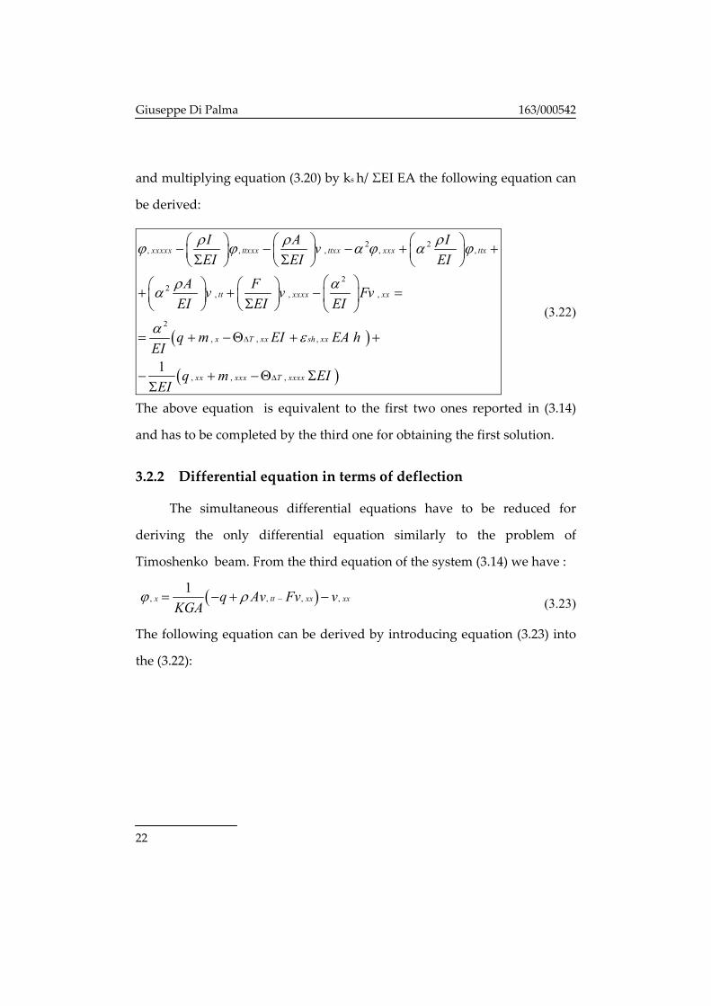
The above equation is equivalent to the first two ones reported in (3.14)
and has to be completed by the third one for obtaining the first solution.
3.2.2 Differential equation in terms of deflection
The simultaneous differential equations have to be reduced for
deriving the only differential equation similarly to the problem of
Timoshenko beam. From the third equation of the system (3.14) we have :
( ), , , ,1
x tt xx xxq Av Fv vKGA
ϕ ρ −= − + − (3.23)
The following equation can be derived by introducing equation (3.23) into
the (3.22):
Page 30
Chapter III ‐ Outline of the governing equations
23
[ ]
[{ ] }
[ ]{
} [ ]
, , , ,
, , , ,
2, , , ,
2, , , , ,
2
1
1
1
1
xxxx ttxxxx xxxxxx xxxxxx
ttxx ttttxx xxxxtt xxxxtt
ttxx xx ttxx xxxx
xxxx tt tttt xxtt xxtt
q Av Fv vKGAI q Av Fv vEI KGAA v q Av FvEI KGA
Iv q Av Fv vEI KGA
AEI
ρ
ρ ρ
ρ α ρ
ρα ρ
ρα
⎧ ⎫− + − − +⎨ ⎬⎩ ⎭
− + − + − − +Σ
− − − + − +Σ
⎧ ⎫− + − + − − +⎨ ⎬⎩ ⎭
+
( )
( )
2
, , ,
2
, , ,
, , ,1
tt xxxx xx
x T xx sh xx
xx xxx T xxxx
Fv v FvEI EI
q m EI EA hEI
q m EIEI
α
α ε∆
∆
+ − =Σ
= + −Θ + +
− + −Θ ΣΣ
(3.24)
A few easy simplifications lead to the following equation in terms of
deflection:
, ,
2 2
, ,
2 2, ,
2,
1 1
1
1
xxxxxx xxxxtt
ttttxx xxtt
tttt tt
xxxx
F A I Fv vKGA KGA EI KGA
A I A A I Fv vKGA EI EI KGA EI KGA
A I Av vKGA EI EI
F FvKGA EI
ρ ρ
ρ ρ ρ α ρ α ρ
ρ ρ ρα α
α
⎡ ⎤⎛ ⎞ ⎛ ⎞+ − + + +⎜ ⎟ ⎜ ⎟⎢ ⎥Σ⎝ ⎠ ⎝ ⎠⎣ ⎦⎡ ⎤⎛ ⎞ ⎛ ⎞+ + + + +⎜ ⎟ ⎜ ⎟⎢ ⎥Σ Σ⎝ ⎠ ⎝ ⎠⎣ ⎦
⎛ ⎞ ⎛ ⎞− − +⎜ ⎟ ⎜ ⎟⎝ ⎠ ⎝ ⎠⎡ ⎛ ⎞− + +⎜ ⎟⎢ Σ⎝ ⎠⎣
( )
( )
2,
2
, , ,
, , ,
2, , , ,
1
1
xx
x T xx sh xx
xx xxx T xxxx
xxxx xx ttxx tt
FvEI
q m EI EA hEI
q m EIEI
I Iq q q qKGA EI EI
α
α ε
ρ ρα
∆
∆
⎤+ =⎥
⎦
= − + −Θ + +
+ + −Θ Σ +Σ
⎛ ⎞− − − +⎜ ⎟Σ⎝ ⎠
(3.25)
Page 31
Giuseppe Di Palma 163/000542
24
The above equation represents in the dynamic field the equation of the
deflection in presence of the constant axial force and of the finite shear
stiffness ( that is F≠0 and [(KGA L2)/EI] ≠ ∞).
In the static field the above equation is simplified as follows:
( )
( ) ( )
2 2, , ,
2
, , ,
2, , , , ,
1 1
1 1
xxxxxx xxxx xx
x T xx sh xx
xx xxx T xxxx xxxx xx
F F F Fv v vKGA KGA EI EI
q m EI EA hEI
q m EI q qEI KGA
α α
α ε
α
∆
∆
⎡ ⎤⎛ ⎞ ⎛ ⎞+ − + + + =⎜ ⎟ ⎜ ⎟⎢ ⎥Σ⎝ ⎠ ⎝ ⎠⎣ ⎦
= − + −Θ + +
+ + −Θ Σ − −Σ
(3.26)
As the axial force F=0 , the following equation can be derived:
( )
( ) ( )
22
, , , , ,
2, , , , ,
1 1
xxxxxx xxxx x T xx sh xx
xx xxx T xxxx xxxx xx
v v q m EI EAhEI
q m EI q qEI KGA
αα ε
α
∆
∆
− = − + −Θ + +
+ + −Θ Σ − −Σ
(3.27)
If no shear flexibility is assumed, the Timoshenko equation usually reduces
to the Bernoulli’s one and the following equation can be obtained as F=0:
( )
( )
22
, , , , ,
, , ,1
xxxxxx xxxx x T xx sh xx
xx xxx T xxxx
v v q m EI EAhEI
q m EIEI
αα ε∆
∆
− = − + −Θ + +
+ + −Θ ΣΣ
(3.28)
Finally, equation (3.28) reduces to the usual differential equation of the
Bernoulli beam as a completely stiff connection is considered ( Lα →∞ ) :
( ), , , ,1
xxxx x T xx sh xxv q m EI EAhEI
ε∆= + −Θ + (3.29)
Page 32
Chapter III ‐ Outline of the governing equations
25
while, as absent connection occurs ( 0Lα → ), the equation of the beam
with flexural stiffness ΣEI is obtained:
( ), , , ,1
xxxxxx xx xxx T xxxxv q m EIEI
∆= + −Θ ΣΣ
(3.30)
As concrete slab is connected to steel beam , for Lα →∞ , shrinkage axial
deformation causes the bending moment . Therefore, such shrinkage axial
deformation appears in the equation of bending (3.29). However, no
bending moment arises by shrinkage in concrete for the case of 0Lα → .
As a result, shrinkage axial deformation freely occurs in concrete slab
(which is not constrained by steel beam through any friction or connection)
and it does not appear in equation of the flexion.
3.2.3 Deriving the other parameters
The following statements are valid only in the static field .
Equation (2.19) in terms of bending moment M can be transformed as
follows:
Page 33
Giuseppe Di Palma 163/000542
26
, ,2 2
, ,
, , ,, ,
,2 , 1
sxx xx T
s
s xx xx s sh s T
xx T xx xxxxx xxxx
xxxxxx
s
q F hEA F kM EI v vKGA KGA k E A
q Fk h v v k k hKGA KGA
EI q F EI m qv vh KGA KGA h h hFv EA EI FFy vh k KGA
v
ε
∆
∆
∆
⎛ ⎞ ⎡= Σ − − − −Θ − +⎜ ⎟ ⎢⎝ ⎠ ⎣⎛ ⎞− − − − − + Θ +⎜ ⎟⎝ ⎠
Σ Σ Θ⎛ ⎞+ − − − − + + +⎜ ⎟⎝ ⎠
⎡ Σ ⎤⎤ ⎛ ⎞+ + = + +⎜ ⎟⎢ ⎥⎥⎦ ⎝ ⎠⎣ ⎦
+
[ ] ( )
2,
2
, ,
22 2
,
1 1xxs
xx xs s s
T sh
T xxs
F F EA FEI EAhKGA KGA k
EI EAh EA EI EA EAq q mKGA KGA k KGA k k
F EA hF Fy EI EA hE A
EI EAk
ε∆
∆
⎡ ⎤⎛ ⎞ ⎛ ⎞−Σ + − + − +⎜ ⎟ ⎜ ⎟⎢ ⎥⎝ ⎠ ⎝ ⎠⎣ ⎦⎡ ⎤ ⎡ ⎤Σ Σ ⎛ ⎞+ − − − + + − +⎜ ⎟⎢ ⎥ ⎢ ⎥ ⎝ ⎠⎣ ⎦⎣ ⎦⎡ ⎤+ − + +Θ − + +⎢ ⎥⎣ ⎦
⎡ ⎤Σ+Θ ⎢ ⎥
⎣ ⎦
(3.31)
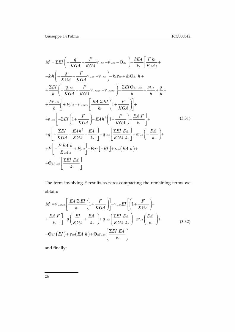
The term involving F results as zero; compacting the remaining terms we
obtain:
( ) ( )
, ,
, ,
,
1 1xxxx xxs
xx xs s s s
T sh T xxs
EA EI F FM v v EIk KGA KGA
EA F EI EA EI EA EAq q mk KGA k KGA k k
EI EAEI EA hk
ε∆ ∆
⎡ Σ ⎤ ⎡⎛ ⎞ ⎛ ⎞= + − + +⎜ ⎟ ⎜ ⎟⎢ ⎥ ⎢⎝ ⎠ ⎝ ⎠⎣ ⎦ ⎣⎛ ⎞Σ⎤ ⎛ ⎞ ⎛ ⎞+ − + + − +⎜ ⎟⎜ ⎟ ⎜ ⎟⎥⎦ ⎝ ⎠ ⎝ ⎠⎝ ⎠
⎛ ⎞Σ−Θ + +Θ ⎜ ⎟
⎝ ⎠
(3.32)
and finally:
Page 34
Chapter III ‐ Outline of the governing equations
27
( )
, ,2 2
, ,2 2 2
,2 2
1 1xxxx xx
xx x
sT sh T xx
EI F F EI FM v v EIKGA KGA EI
EI EI EI EIq q mKGA EI KGA EI
EI k h EIEIEI
α α
α α α
εα α
∆ ∆
⎡ ⎤⎡ ⎤⎛ ⎞ ⎛ ⎞= + − + + +⎜ ⎟ ⎜ ⎟⎢ ⎥⎢ ⎥ Σ⎝ ⎠ ⎝ ⎠⎣ ⎦ ⎣ ⎦⎛ ⎞ ⎛ ⎞ ⎛ ⎞
− + + − +⎜ ⎟ ⎜ ⎟ ⎜ ⎟Σ Σ⎝ ⎠ ⎝ ⎠ ⎝ ⎠⎛ ⎞ ⎛ ⎞−Θ + +Θ⎜ ⎟ ⎜ ⎟Σ ⎝ ⎠⎝ ⎠
(3.33)
The normal stress in concrete slab N1, and the normal stress in the steel
beam N2, are obtained from the following equation which is derived by
substituting (3.23) into (3.16):
1 22 2
, , ,, ,
, , ,
ss sh s T
s
xx xx xxxxs xx xxxx
T xx x xx
EA F kN F N k k hk E A
q Fv EI q Fvk v h vKGA h KGA
EI m q Fvh h h h
ε ∆
∆
⎧= − = − + Θ⎨⎩
+ Σ +⎛ ⎞ ⎛ ⎞− − − + − − +⎜ ⎟ ⎜ ⎟⎝ ⎠ ⎝ ⎠
Σ Θ ⎫− + + + ⎬⎭
(3.34)
that is reorganizing:
,1 2
2 2
2, ,
,
,
1 1
1
s xxs sh s T
T xx x sxxxx
xx s
EI F k EI qN k k hEI E A h KGA
EI F EI m q k hvh KGA h h h KGA
F Fv k hh KGA
εα
∆
∆
⎧ Σ= − + Θ − +⎨Σ ⎩
⎛ ⎞Σ Σ Θ⎛ ⎞− + − + + + +⎜ ⎟⎜ ⎟⎝ ⎠ ⎝ ⎠
⎫⎡ ⎤⎛ ⎞+ + + =⎬⎜ ⎟⎢ ⎥⎝ ⎠⎣ ⎦⎭
(3.35)
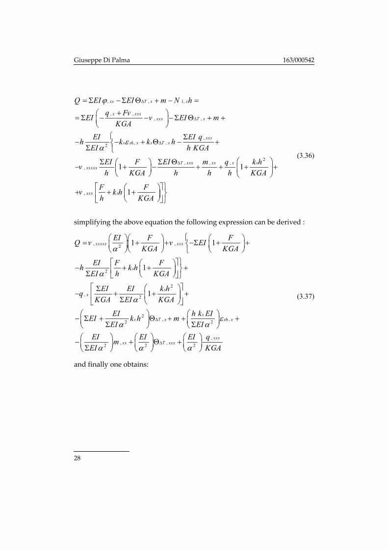
Equation (2.12) can be written in the static field. From this equation Q can
be derived. Substituting equation (3.33) into Q expression one obtains:
Page 35
Giuseppe Di Palma 163/000542
28
, , 1,
, ,, ,
,, ,2
2, , ,
,
,
1 1
1
xx T x x
x xxxxxx T x
xxxs sh x s T x
T xxx xx x sxxxxx
xxx s
Q EI EI m N hq FvEI v EI mKGA
EI EI qh k k hEI h KGA
EI F EI m q k hvh KGA h h h KGA
F Fv k hh KGA
ϕ
εα
∆
∆
∆
∆
= Σ −Σ Θ + − =
+⎛ ⎞= Σ − − −Σ Θ + +⎜ ⎟⎝ ⎠
⎧ Σ− − + Θ − +⎨Σ ⎩
⎛ ⎞Σ Σ Θ⎛ ⎞− + − + + + +⎜ ⎟⎜ ⎟⎝ ⎠ ⎝ ⎠
⎡ ⎛ ⎞+ + +⎜ ⎟⎝ ⎠
⎫⎤⎬⎢ ⎥
⎣ ⎦⎭
(3.36)
simplifying the above equation the following expression can be derived :
, ,2
2
2
, 2
2, ,2 2
2
1 1
1
1
xxxxx xxx
s
sx
ss T x sh x
EI F FQ v v EIKGA KGA
EI F Fh k hEI h KGA
EI EI k hqKGA EI KGA
EI h k EIEI k h mEI EI
EIEI
α
α
α
εα α
α
∆
⎧⎛ ⎞⎛ ⎞ ⎛ ⎞= + + −Σ + +⎨⎜ ⎟ ⎜ ⎟⎜ ⎟⎝ ⎠ ⎝ ⎠⎝ ⎠ ⎩⎫⎡ ⎤⎛ ⎞− + + +⎬⎜ ⎟⎢ ⎥Σ ⎝ ⎠⎣ ⎦⎭
⎡ ⎤⎛ ⎞Σ− + + +⎢ ⎥⎜ ⎟Σ ⎝ ⎠⎣ ⎦⎛ ⎞ ⎛ ⎞− Σ + Θ + + +⎜ ⎟ ⎜ ⎟Σ Σ⎝ ⎠ ⎝ ⎠⎛ ⎞−⎜ ⎟Σ⎝ ⎠
,, ,2 2
xxxxx T xxx
EI EI qmKGAα α
∆⎛ ⎞ ⎛ ⎞+ Θ +⎜ ⎟ ⎜ ⎟⎝ ⎠ ⎝ ⎠
(3.37)
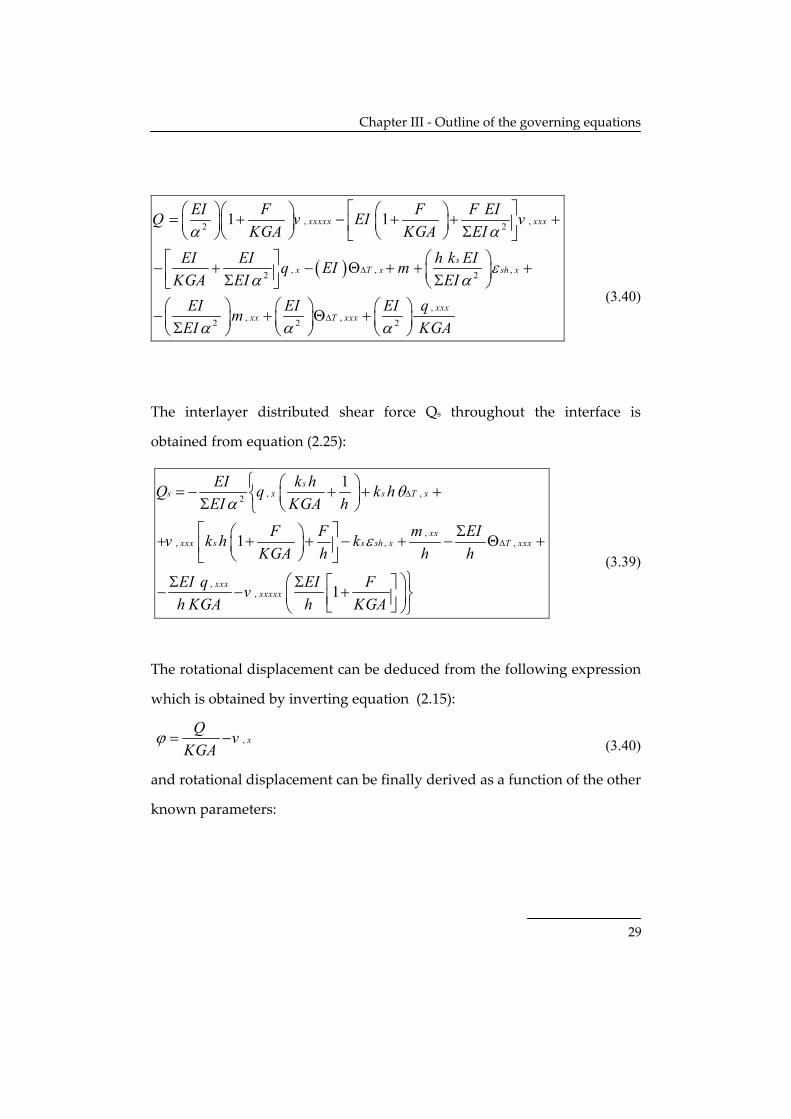
and finally one obtains:
Page 36
Chapter III ‐ Outline of the governing equations
29
( )
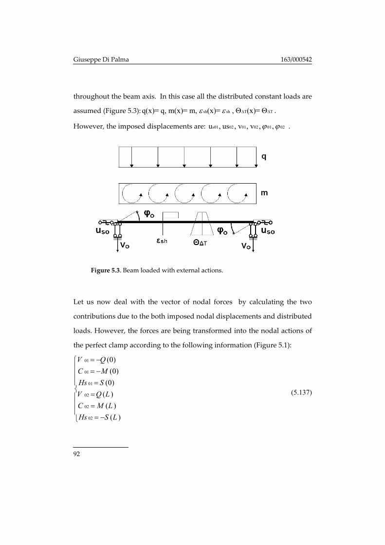
, ,2 2
, , ,2 2
,, ,2 2 2
1 1xxxxx xxx
sx T x sh x
xxxxx T xxx
EI F F F EIQ v EI vKGA KGA EI
EI EI h k EIq EI mKGA EI EIEI EI EI qmEI KGA
α α
εα α
α α α
∆
∆
⎡ ⎤⎛ ⎞⎛ ⎞ ⎛ ⎞= + − + + +⎜ ⎟ ⎜ ⎟⎜ ⎟ ⎢ ⎥Σ⎝ ⎠ ⎝ ⎠⎝ ⎠ ⎣ ⎦⎡ ⎤ ⎛ ⎞− + − Θ + + +⎜ ⎟⎢ ⎥Σ Σ⎣ ⎦ ⎝ ⎠⎛ ⎞ ⎛ ⎞ ⎛ ⎞− + Θ +⎜ ⎟ ⎜ ⎟ ⎜ ⎟Σ⎝ ⎠ ⎝ ⎠ ⎝ ⎠
(3.40)
The interlayer distributed shear force Qs throughout the interface is
obtained from equation (2.25):
, ,2
,, , ,
,,
1
1
1
ss x s T x
xxxxx s s sh x T xxx
xxxxxxxx
EI k hQ q k hEI KGA h
F F m EIv k h kKGA h h h
EI q EI Fvh KGA h KGA
θα
ε
∆
∆
⎧ ⎛ ⎞= − + + +⎨ ⎜ ⎟Σ ⎝ ⎠⎩⎡ ⎤ Σ⎛ ⎞+ + + − + − Θ +⎜ ⎟⎢ ⎥⎝ ⎠⎣ ⎦
⎫Σ ⎛ Σ ⎞⎡ ⎤− − + ⎬⎜ ⎟⎢ ⎥⎣ ⎦⎝ ⎠⎭
(3.39)
The rotational displacement can be deduced from the following expression
which is obtained by inverting equation (2.15):
, xQ vKGA
ϕ = − (3.40)
and rotational displacement can be finally derived as a function of the other
known parameters:
Page 37
Giuseppe Di Palma 163/000542
30
( )
, ,2
,,2 2
, , ,
2 2
, ,
2
1 1xxxxx xxx
xx
xxx xx T x
sh x s T xxx
EI F EI Fv vKGA KGA KGA KGA
EI F q EI EIvEI KGA KGA KGA EI
q EI m m EI EIKGA KGA KGA KGA EI KGA
EI k h EIKGA EI KGA
ϕα
α α
α α
εα α
∆
∆
⎛ ⎞ ⎛⎡ ⎤ ⎡ ⎤= + − + +⎜ ⎟ ⎜⎢ ⎥ ⎢ ⎥⎣ ⎦ ⎣ ⎦⎝⎝ ⎠⎞ ⎛ ⎞+ − − + +⎟ ⎜ ⎟Σ Σ⎝ ⎠⎠
⎛ ⎞ Θ⎛ ⎞+ + − − +⎜ ⎟ ⎜ ⎟Σ⎝ ⎠⎝ ⎠Θ
+ +Σ 2
⎛ ⎞⎜ ⎟⎝ ⎠
(3.41)
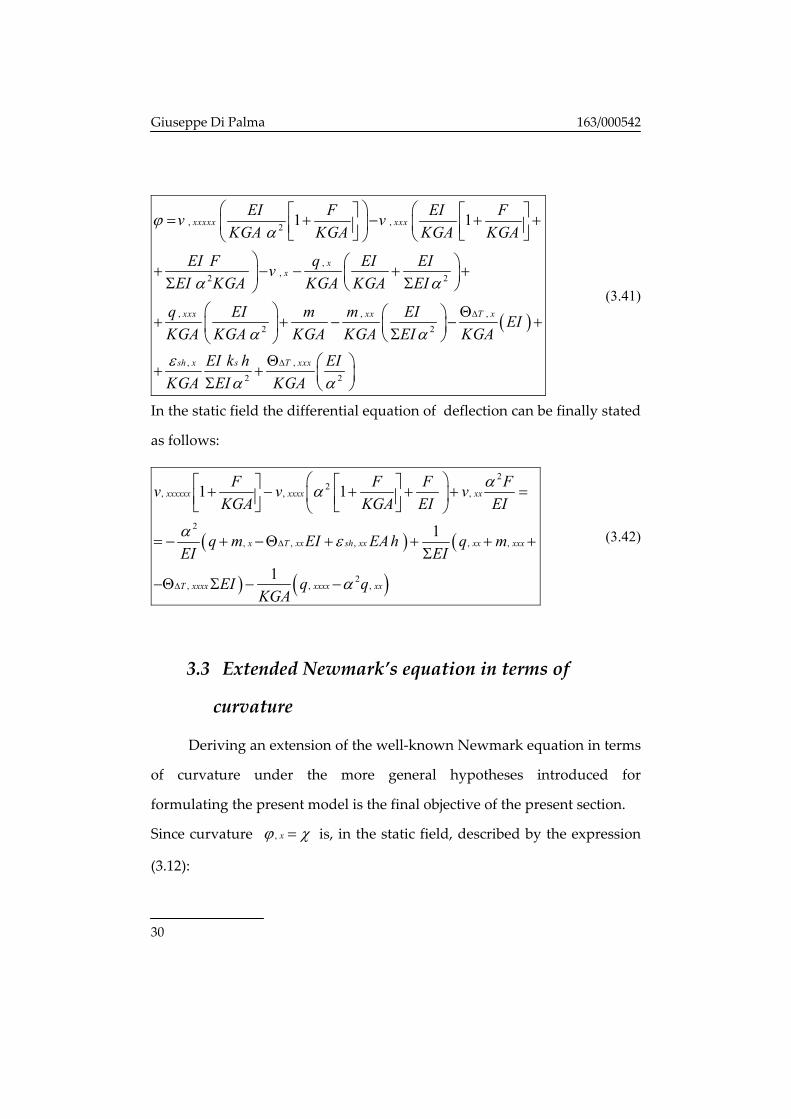
In the static field the differential equation of deflection can be finally stated
as follows:
( ) (
) ( )
22
, , ,
2
, , , , ,
2, , ,
1 1
1
1
xxxxxx xxxx xx
x T xx sh xx xx xxx
T xxxx xxxx xx
F F F Fv v vKGA KGA EI EI
q m EI EAh q mEI EI
EI q qKGA
αα
α ε
α
∆
∆
⎛ ⎞⎡ ⎤ ⎡ ⎤+ − + + + =⎜ ⎟⎢ ⎥ ⎢ ⎥⎣ ⎦ ⎣ ⎦⎝ ⎠
= − + −Θ + + + +Σ
−Θ Σ − −
(3.42)
3.3 Extended Newmark’s equation in terms of
curvature
Deriving an extension of the well‐known Newmark equation in terms
of curvature under the more general hypotheses introduced for
formulating the present model is the final objective of the present section.
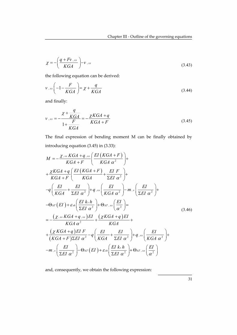
Since curvature , xϕ χ= is, in the static field, described by the expression
(3.12):
Page 38
Chapter III ‐ Outline of the governing equations
31
,,
xxxx
q Fv vKGA
χ +⎛ ⎞= − −⎜ ⎟⎝ ⎠
(3.43)
the following equation can be derived:
, 1xxF qvKGA KGA
χ⎛ ⎞− − = +⎜ ⎟⎝ ⎠
(3.44)
and finally:
,
1xx
qKGA qKGAv F KGA F
KGA
χ χ+ += − = −
++ (3.45)
The final expression of bending moment M can be finally obtained by
introducing equation (3.45) in (3.33):
( )
( )
( )
( )
, ,
2
2
, ,2 2 2
,2 2
, ,
2
xx xx
xx x
sT sh T xx
xx xx
EI KGA FKGA qMKGA F KGA
EI KGA FKGA q EI FKGA F KGA EI
EI EI EI EIq q mKGA EI KGA EI
EI k h EIEIEI
KGA q EIKGA
χα
χα
α α α
εα α
χα
∆ ∆
+⎛ ⎞+= − +⎜ ⎟+ ⎝ ⎠
+⎛ ⎞++ + +⎜ ⎟+ Σ⎝ ⎠
⎛ ⎞ ⎛ ⎞ ⎛ ⎞− + + − +⎜ ⎟ ⎜ ⎟ ⎜ ⎟Σ Σ⎝ ⎠ ⎝ ⎠ ⎝ ⎠
⎛ ⎞ ⎛ ⎞−Θ + +Θ =⎜ ⎟ ⎜ ⎟Σ ⎝ ⎠⎝ ⎠+
= − +( )
( )( )
( )
,2 2 2
, ,2 2 2
xx
sx T sh T xx
KGA q EIKGA
KGA q EI F EI EI EIq qKGA F EI KGA EI KGA
EI EI k h EIm EIEI EI
χ
χα α α
εα α α
∆ ∆
++
+ ⎛ ⎞ ⎛ ⎞+ − + + +⎜ ⎟ ⎜ ⎟+ Σ Σ⎝ ⎠ ⎝ ⎠
⎛ ⎞ ⎛ ⎞ ⎛ ⎞− −Θ + +Θ⎜ ⎟ ⎜ ⎟ ⎜ ⎟Σ Σ ⎝ ⎠⎝ ⎠ ⎝ ⎠
(3.46)
and, consequently, we obtain the following expression:
Page 39
Giuseppe Di Palma 163/000542
32
( ) ( )
( )
,,2 2
2 2
, ,2 2 2
,2 2
xxxx
xx x
sT sh T xx
EI EI EIM q EI qKGA KGA
KGA EI F q EI FKGA F EI KGA F EI
EI EI EI EIq q mKGA EI KGA EI
EI k h EIEIEI
χ χα α
χα α
α α α
εα α
∆ ∆
= − − + + +
+ + ++ Σ + Σ
⎛ ⎞ ⎛ ⎞ ⎛ ⎞− + + − +⎜ ⎟ ⎜ ⎟ ⎜ ⎟Σ Σ⎝ ⎠ ⎝ ⎠ ⎝ ⎠
⎛ ⎞ ⎛ ⎞−Θ + +Θ⎜ ⎟ ⎜ ⎟Σ ⎝ ⎠⎝ ⎠
(3.47)
Therefore, multiplying (3.47) by ( )2 KGA F EIα + Σ we obtain:
( ) ( )
( ) ( )
( ) ( )
,,
2 2
, ,2 2 2
2,2 2
xxxx
xx x
sT sh T xx
q EIEI KGA F EI KGA F EIKGAq EIEI KGA F EI KGA F EIKGA
KGA EI F q EI F
EI EI EI EIq q mKGA EI KGA EI
EI k h EIEI KGA F EIEI
χ
χ α α
χ
α α α
ε αα α
∆ ∆
− + Σ − + Σ +
+ + Σ + + Σ +
+ + +
⎧ ⎛ ⎞ ⎛ ⎞ ⎛ ⎞⎪− + + − +⎨ ⎜ ⎟ ⎜ ⎟ ⎜ ⎟Σ Σ⎪ ⎝ ⎠ ⎝ ⎠ ⎝ ⎠⎩⎫⎛ ⎞ ⎪⎛ ⎞−Θ + +Θ + Σ⎬⎜ ⎟ ⎜ ⎟Σ ⎝ ⎠⎪⎝ ⎠ ⎭
( ) 2M KGA F EI α
=
= + Σ
(3.48)
and finally one obtains:
Page 40
Chapter III ‐ Outline of the governing equations
33
( ) ( )
( ) ( )
( )
( ) ( )
2,
2,
,2 2
, 2 2
2, 2
xx
xx
xx
sx T sh
T xx
EI KGA F EI KGA EI F
q EI q EI EIKGA F EI KGA FKGA KGA
EI EI EIq EI F q qKGA EI KGA
EI EI k hm EIEI EI
EI KGA F EI M KGA F EI
χ α χ χ
α
α α
εα α
α αα
∆
∆
− + Σ − =
Σ= − + Σ + + +
⎧ ⎛ ⎞ ⎛ ⎞⎪+ + − + + +⎨ ⎜ ⎟ ⎜ ⎟Σ⎪ ⎝ ⎠ ⎝ ⎠⎩⎛ ⎞ ⎛ ⎞
− −Θ + +⎜ ⎟ ⎜ ⎟Σ Σ⎝ ⎠ ⎝ ⎠⎫⎛ ⎞+Θ + Σ − + Σ⎬⎜ ⎟
⎝ ⎠⎭
( )
( )
2
2, ,
22
,,2 2 2
2 2,2 2
xx xx
xxx T
ssh T xx
EI F EIq EI EI q q EI EIKGA
q EI EI F qEIq EI F KGA F EIKGA KGA
q EI q EI EIm EIEI KGA EI
EI k h EI M KGA EI M EI FEI
α
α α
α α α
ε α αα α
∆
∆
=
Σ= − Σ − + Σ +
Σ ⎡+ + + + Σ − +⎢⎣
− + − −Θ +Σ Σ
⎤⎛ ⎞ ⎛ ⎞+ +Θ − Σ − Σ⎥⎜ ⎟ ⎜ ⎟Σ ⎝ ⎠⎝ ⎠ ⎦
(3.49)
Hence, the following equation in terms of curvature can be finally derived
for the shear‐flexible composite beams:
( ) ( )
( )
( )
2,
, ,
2
2, ,
1
1
xx
x T xx
sh
shx T xx T
EI KGA F KGA F
KGA EI q m EIEI
M EA hTEI EI
M EA hF EI m EIEI EI EI
χ α χ χ
εα
εα
∆
∆ ∆
− Σ + − =
⎡= − Σ + −Θ Σ +⎢Σ⎣⎤⎛ ⎞+ +Θ∆ − +⎜ ⎟⎥⎝ ⎠⎦
⎡ ⎤⎛ ⎞− Σ −Θ Σ + +Θ −⎜ ⎟⎢ ⎥Σ ⎝ ⎠⎣ ⎦
(3.50)
Page 41
Giuseppe Di Palma 163/000542
34
Such an equation extends the one reported by Faella et al. [25] based on the
work by Newmark et al. [2].
The above equation turns into the standard one as F=0 :
( )2, , ,
2
1xx x T xx
shT
q m EIEI
M EA hEI EI
χ α χ
εα
∆
∆
− = − + −Θ Σ +Σ
⎛ ⎞− +Θ −⎜ ⎟⎝ ⎠
(3.51)
which represents Newmark equation supposing that the shear stiffness is
finite (Timoshenko model).
Such equation takes into account the presence of the following loads:
• distributed vertical load
• distributed bending moment
• shrinkage axial deformation
• thermal induced anelastic strain.
The effect of the shear flexibility , in the equation (3.51), is present in the
definition of the curvature (3.43).
Finally, the equation (describing the curvature of the beam with the
flexural stiffness EI) is obtained on the condition that the connection has its
infinite rigidity ( Lα →∞ ). In concrete slab shrinkage axial deformation is
present resulting in the consequent bending moment:
shT
M EA hEI EI
εχ ∆⎛ ⎞= +Θ −⎜ ⎟⎝ ⎠
(3.52)
If connection has zero stiffness ( 0Lα → ) the following condition can be
easily derived and assured:
Page 42
Chapter III ‐ Outline of the governing equations
35
( ), , ,1
xx x T xxq m EIEI
χ ∆= − + −Θ ΣΣ
(3.53)
Even here we observe that for Lα →∞ the shrinkage axial deformation is
also present in curvature equation, while for 0Lα → such a shrinkage
axial deformation does not result in curvatures, but only in relative
displacements.
Page 43
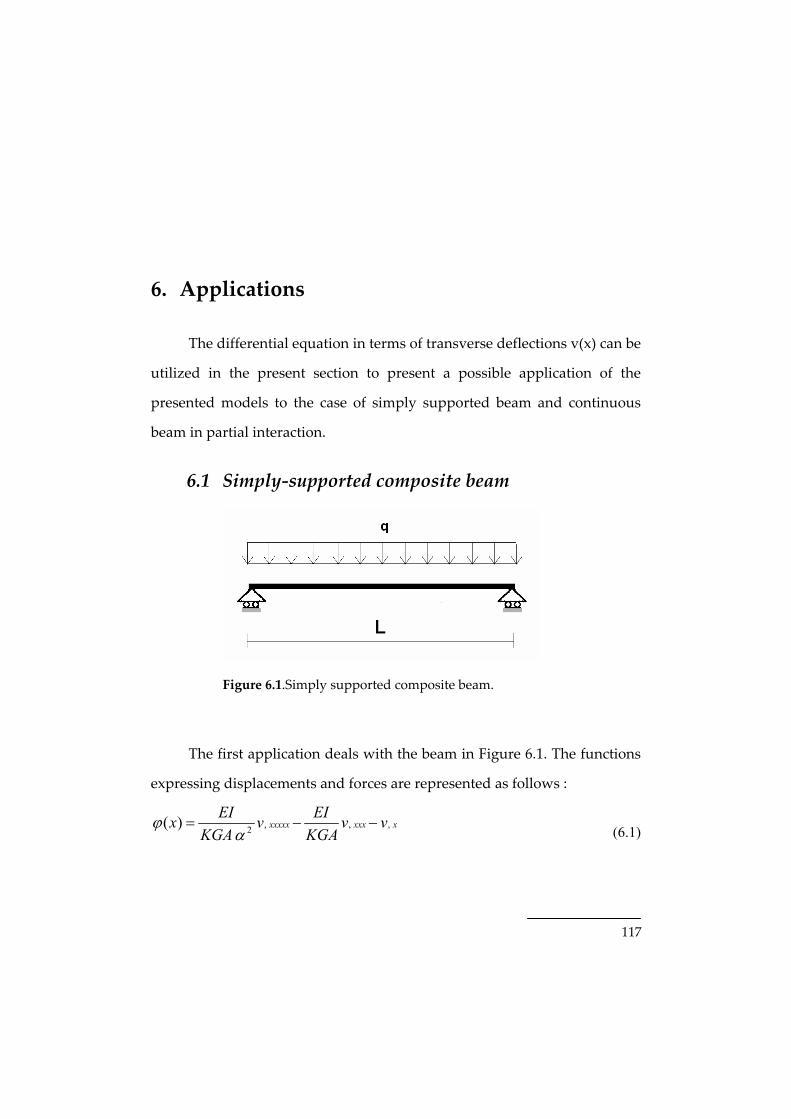
36
4. Solution in the elastic range
The equation formulated in the previous sections will be solved
within the linear range. General boundary and restraint conditions will be
considered throughout the present chapter.
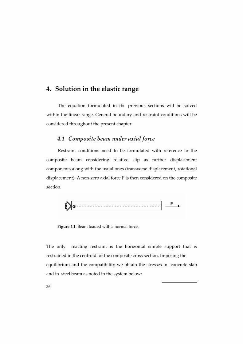
4.1 Composite beam under axial force
Restraint conditions need to be formulated with reference to the
composite beam considering relative slip as further displacement
components along with the usual ones (transverse displacement, rotational
displacement). A non‐zero axial force F is then considered on the composite
section.
Figure 4.1. Beam loaded with a normal force.
The only reacting restraint is the horizontal simple support that is
restrained in the centroid of the composite cross section. Imposing the
equilibrium and the compatibility we obtain the stresses in concrete slab
and in steel beam as noted in the system below:
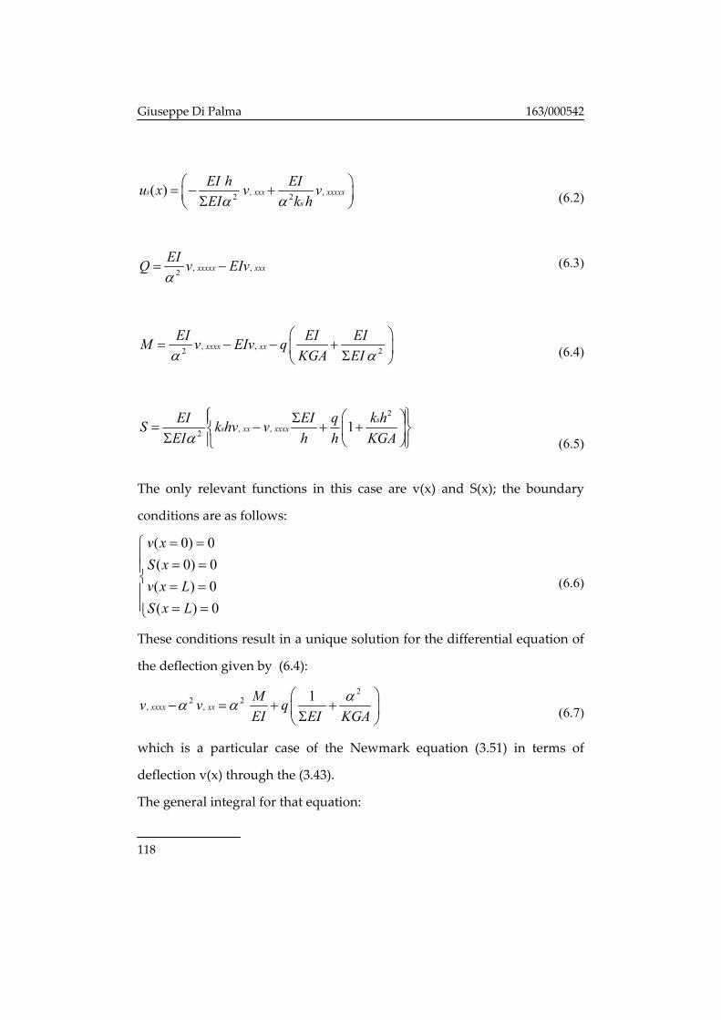
Page 44
Chapter IV ‐ Solution in the elastic range
37
1 21 1 2 2
1 21 21 1 2 2 1 1 2 2
1 1 2 2
,N N F
E A E AN F N FN N E A E A E A E AE A E A
+ =⎧⎪ ⇒ = =⎨ + +=⎪⎩
(4.1)
Consequently, no relative slips occur as an axial force F is applied on the
composite section and shared into the two parts N1 and N2 related to
concrete slab and steel beam respectively.
4.2 Composite beam in bending
Before analysing the bending problem, we should observe that the
composite beam kinematics is based on one more parameter in comparison
with a simple beam.
The kinematic quantity us finds its static counterpart in the mutual reaction
of the dual restraint: horizontal mutual pendulum between the concrete
slab and the steel beam. The bending problem is approached in this section.
The simultaneous equations (3.14) involve three unknowns, namely
deflection v(x) , rotational displacement φ(x) and normal stress N1(x).
In particular, it results that N1(x)=‐N2(x) as F=0.
Consequently the “slip force” S(x) can be considered as a new stress,
perfectly dual of the slip between two parts of the section. The above
definition conceptually simplifies and complete the correspondence
between nodal force S and displacement us.
Page 45
Giuseppe Di Palma 163/000542
38
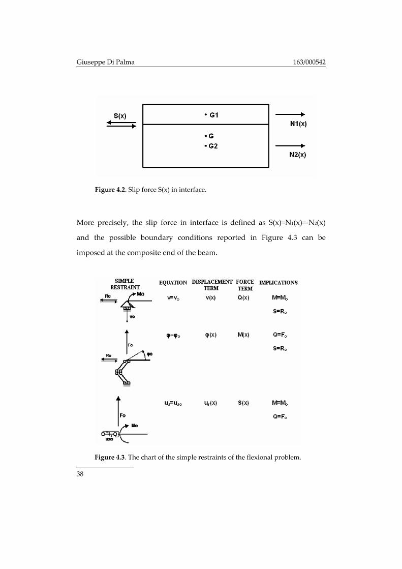
Figure 4.2. Slip force S(x) in interface.
More precisely, the slip force in interface is defined as S(x)=N1(x)=‐N2(x)
and the possible boundary conditions reported in Figure 4.3 can be
imposed at the composite end of the beam.
Figure 4.3. The chart of the simple restraints of the flexional problem.
Page 46
Chapter IV ‐ Solution in the elastic range
39
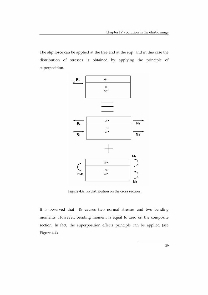
The slip force can be applied at the free end at the slip and in this case the
distribution of stresses is obtained by applying the principle of
superposition.
Figure 4.4. R0 distribution on the cross section .
It is observed that R0 causes two normal stresses and two bending
moments. However, bending moment is equal to zero on the composite
section. In fact, the superposition effects principle can be applied (see
Figure 4.4).
Page 47
Giuseppe Di Palma 163/000542
40
1
2
''
o
o
N RN R
=⎧⎨ = −⎩
(4.2)
1 21 1 2 2
1 21 2
1 1 2 2
'' , ''o
o o
M M R hE I E IM R h M R hM M EI EI
E I E I
+ =⎧⎪ ⇒ = =⎨ Σ Σ=⎪⎩
(4.3)
Consequently the stresses in the cross section can be obtained as follows:
1 1 1
2 2 2
1 1 1 11 1 1
2 2 2 22 2 2
' '' 0' '' 0
' '' 0
' '' 0
o o
o o
o o
o o
N N N R RN N N R R
E I E IM M M R h R hEI EIE I E IM M M R h R hEI EI
= + = + == + = − + = −
= + = + =Σ Σ
= + = + =Σ Σ
(4.4)
The bending moment is equal to 0 as it has been stated before :
1 1 2 2
1 2 1 0o o oE I E IM M M N h R h R h R hEI EI
= + − = + − =Σ Σ
(4.5)
4.2.1 Non‐redundant beams in bending
In case of simply supported beams the bending moment is always
known throughout equilibrium. This bending moment results by q(x),
m(x), as well as by the nodal forces M0 and F0. The shrinkage axial
deformation and thermal curvature as well as the restraint displacements
do not result in the stresses being the non‐redundant beam.
Therefore subsists the following equation:
Page 48
Chapter IV ‐ Solution in the elastic range
41
0 0 0( , , , , )( ) 0sh T sv uM x ε ϕ∆Θ = (4.6)
Consequently, the total bending moment M(x) can be obtained as follows :
( ) ( )( ) ( ) ( ) ( ) ( )q x m x Mo FoM x M x M x M x M x= + + + (4.7)
and is always known a priori. The equation in terms of bending moments
can be applied:
, ,2 2
, , ,2 2 2 2
xxxx xx
sxx x T sh T xx
EI EI EIM v v EI qKGA EI
EI EI EI k h EIq m EIKGA EI EI
α α
εα α α α
∆ ∆
⎛ ⎞= − − + +⎜ ⎟Σ⎝ ⎠
+ − −Θ + +ΘΣ Σ
(4.8)
which can be solved against deflection v(x) as follows:
( ) ( )
2 2, ,
2, , ,
1 1
shxxxx xx T
x T xx xx
M EA hv vEI EI
q m EI q qEI KGA
εα α
α
∆
∆
⎛ ⎞− = +Θ −⎜ ⎟
⎝ ⎠
+ + −Θ Σ + −Σ
(4.9)
the general integral is:
1 2 3 4( ) ( ) cosh( ) ( )pv x C senh x C x C x C v xα α= + + + + (4.10) being vp(x) a peculiar integral of the complete equation which can be
founded on condition that the functions M(x) as well as the static and
kinematic loads are known, and :
C1, C2, C3 and C4 are the integration constants obtainable by four
boundary conditions.
Page 49
Giuseppe Di Palma 163/000542
42
4.2.2 Boundary conditions for non‐redundant beams
The integration constants can be derived by imposing the relevant
boundary conditions deriving from the restraints.
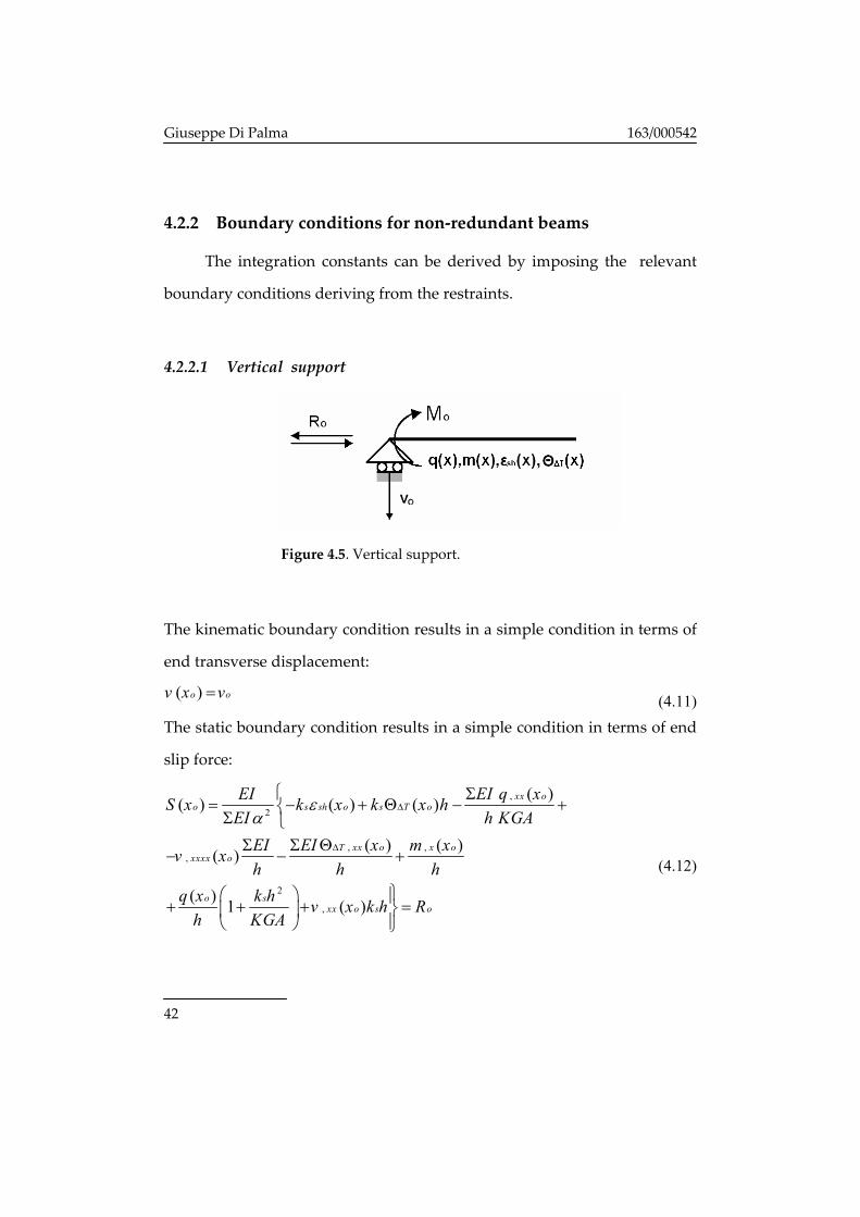
4.2.2.1 Vertical support
Figure 4.5. Vertical support.
The kinematic boundary condition results in a simple condition in terms of
end transverse displacement:
( )o ov x v= (4.11) The static boundary condition results in a simple condition in terms of end
slip force:
,
2
, ,,
2
,
( )( ) ( ) ( )
( ) ( )( )
( ) 1 ( )
xx oo s sh o s T o
T xx o x oxxxx o
o sxx o s o
EI EI q xS x k x k x hEI h KGAEI EI x m xv xh h h
q x k h v x k h Rh KGA
εα
∆
∆
⎧ Σ= − + Θ − +⎨Σ ⎩
Σ Σ Θ− − +
⎫⎛ ⎞ ⎪+ + + =⎬⎜ ⎟⎪⎝ ⎠ ⎭
(4.12)
Page 50
Chapter IV ‐ Solution in the elastic range
43
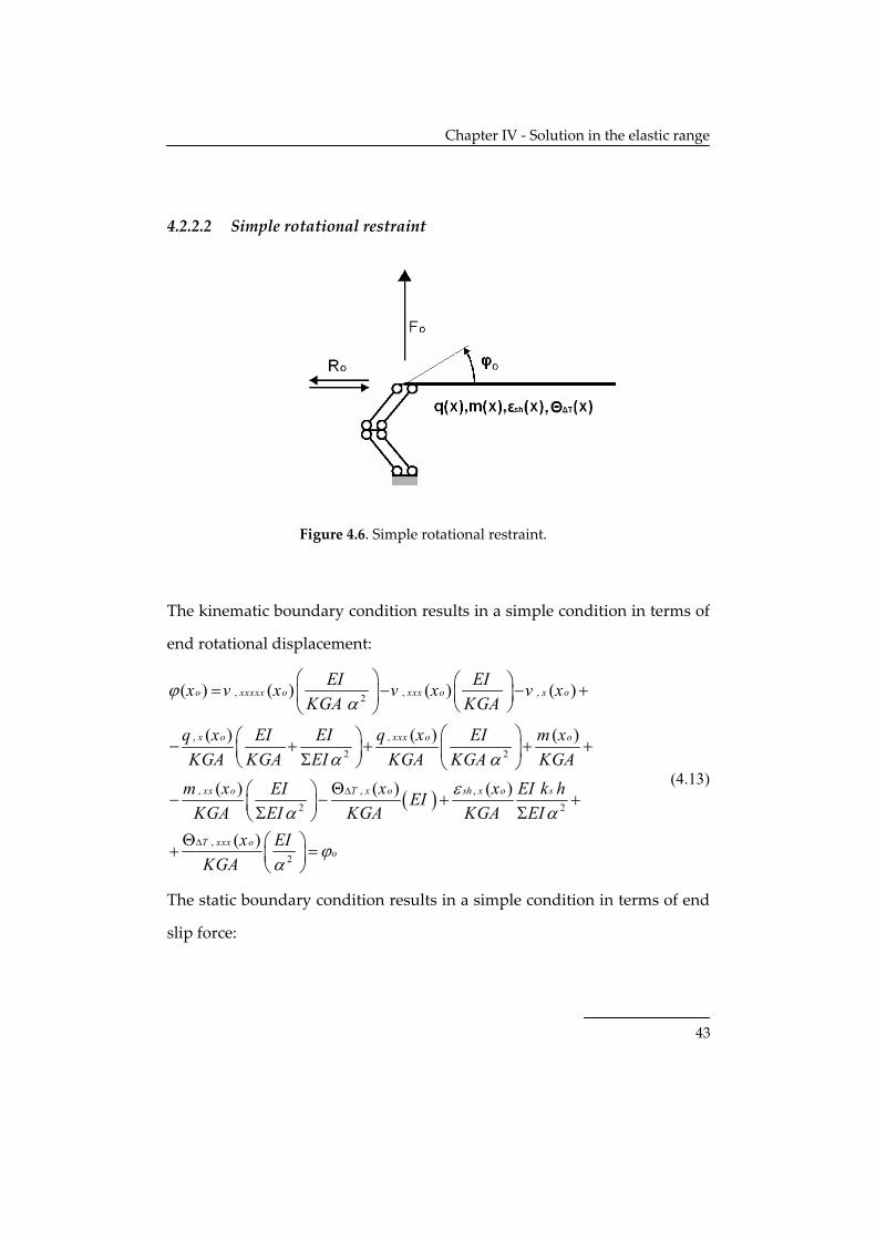
4.2.2.2 Simple rotational restraint
Figure 4.6. Simple rotational restraint.
The kinematic boundary condition results in a simple condition in terms of
end rotational displacement:
( )
, , ,2
, ,
2 2
, , ,
2 2
,
( ) ( ) ( ) ( )
( ) ( ) ( )
( ) ( ) ( )
(
o xxxxx o xxx o x o
x o xxx o o
xx o T x o sh x o s
T xxx
EI EIx v x v x v xKGA KGA
q x EI EI q x EI m xKGA KGA EI KGA KGA KGA
m x EI x x EI k hEIKGA EI KGA KGA EI
x
ϕα
α α
εα α
∆
∆
⎛ ⎞ ⎛ ⎞= − − +⎜ ⎟ ⎜ ⎟⎝ ⎠⎝ ⎠
⎛ ⎞⎛ ⎞− + + + +⎜ ⎟⎜ ⎟Σ⎝ ⎠ ⎝ ⎠Θ⎛ ⎞− − + +⎜ ⎟Σ Σ⎝ ⎠
Θ+ 2
)oo
EIKGA
ϕα
⎛ ⎞ =⎜ ⎟⎝ ⎠
(4.13)
The static boundary condition results in a simple condition in terms of end
slip force:
Page 51
Giuseppe Di Palma 163/000542
44
}
,
2
2, ,
,
,
( )( ) ( ) ( )
( ) ( ) ( )( ) 1
( )
xx oo s sh o s T o
T xx o x o o sxxxx o
xx o s o
EI EI q xS x k x k x hEI h KGA
EI EI x m x q x k hv xh h h h KGA
v x k h R
εα
∆
∆
⎧ Σ= − + Θ − +⎨Σ ⎩
⎛ ⎞Σ Σ Θ− − + + + +⎜ ⎟
⎝ ⎠+ =
(4.14)
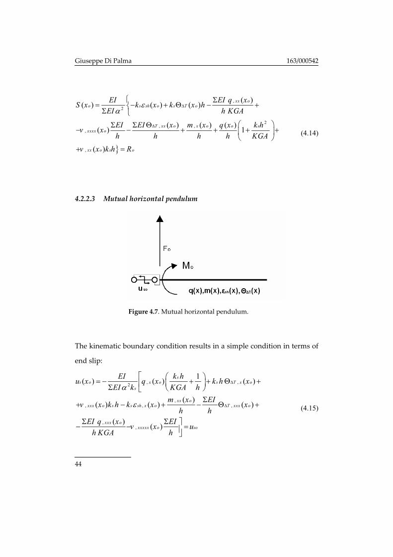
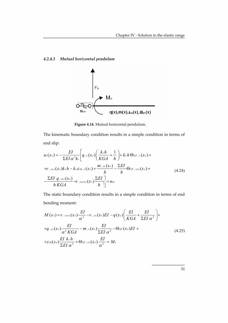
4.2.2.3 Mutual horizontal pendulum
Figure 4.7. Mutual horizontal pendulum.
The kinematic boundary condition results in a simple condition in terms of
end slip:
, ,2
,, , ,
,,
1( ) ( ) ( )
( )( ) ( ) ( )
( ) ( )
ss o x o s T x o
s
xx oxxx o s s sh x o T xxx o
xxx oxxxxx o so
EI k hu x q x k h xEI k KGA h
m x EIv x k h k x xh h
EI q x EIv x uh KGA h
α
ε
∆
∆
⎡ ⎛ ⎞= − + + Θ +⎜ ⎟⎢Σ ⎝ ⎠⎣Σ
+ − + − Θ +
Σ Σ ⎤− − =⎥⎦
(4.15)
Page 52
Chapter IV ‐ Solution in the elastic range
45
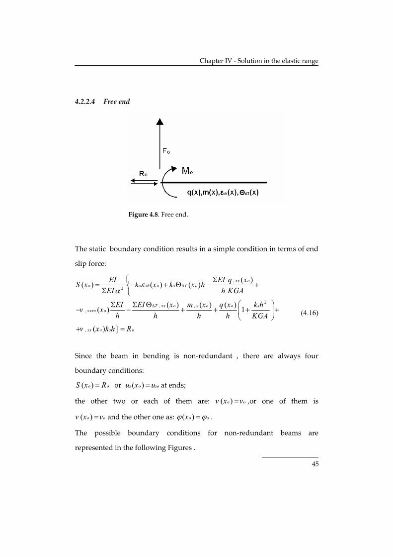
4.2.2.4 Free end
Figure 4.8. Free end.
The static boundary condition results in a simple condition in terms of end
slip force:
}
,
2
2, ,
,
,
( )( ) ( ) ( )
( ) ( ) ( )( ) 1
( )
xx oo s sh o s T o
T xx o x o o sxxxx o
xx o s o
EI EI q xS x k x k x hEI h KGA
EI EI x m x q x k hv xh h h h KGA
v x k h R
εα
∆
∆
⎧ Σ= − + Θ − +⎨Σ ⎩
⎛ ⎞Σ Σ Θ− − + + + +⎜ ⎟
⎝ ⎠+ =
(4.16)
Since the beam in bending is non‐redundant , there are always four
boundary conditions:
( )o oS x R= or ( )s o sou x u= at ends;
the other two or each of them are: ( )o ov x v= ,or one of them is
( )o ov x v= and the other one as: ( )o oxϕ ϕ= .
The possible boundary conditions for non‐redundant beams are
represented in the following Figures .
Page 53
Giuseppe Di Palma 163/000542
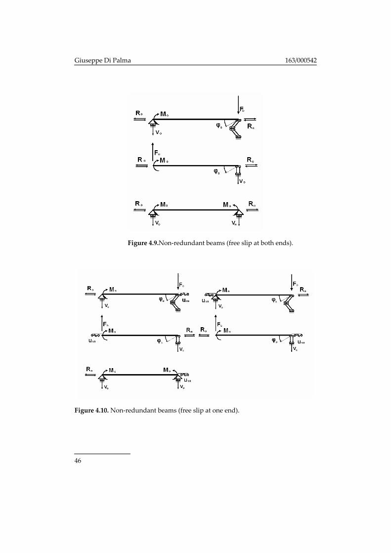
46
Figure 4.9.Non‐redundant beams (free slip at both ends).
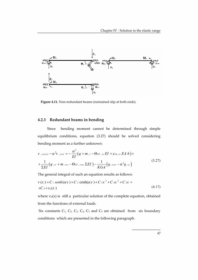
Figure 4.10. Non‐redundant beams (free slip at one end).
Page 54
Chapter IV ‐ Solution in the elastic range
47
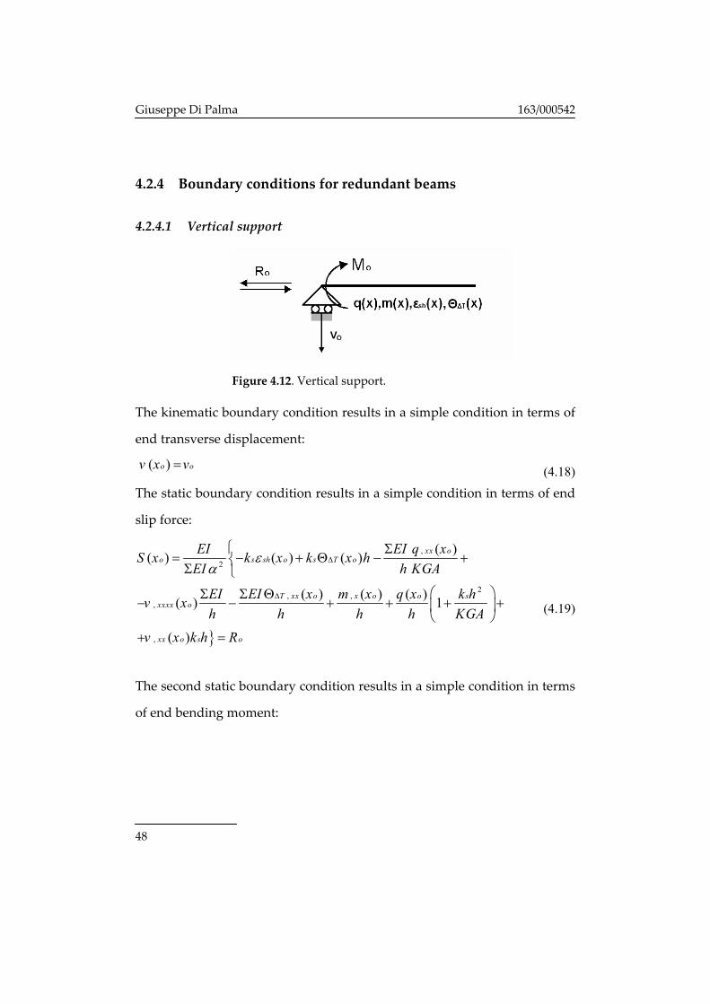
Figure 4.11. Non‐redundant beams (restrained slip at both ends).
4.2.3 Redundant beams in bending
Since bending moment cannot be determined through simple
equilibrium conditions, equation (3.27) should be solved considering
bending moment as a further unknown:
( )
( ) ( )
22
, , , , ,
2, , , , ,
1 1
xxxxxx xxxx x T xx sh xx
xx xxx T xxxx xxxx xx
v v q m EI EA hEI
q m EI q qEI KGA
αα ε
α
∆
∆
− = − + −Θ + +
+ + −Θ Σ − −Σ
(3.27)
The general integral of such an equation results as follows: 3 2
1 2 3 4 5
6
( ) ( ) cosh( )( )p
v x C senh x C x C x C x C xC v x
α α= + + + + ++ +
(4.17)
where vp(x) is still a particular solution of the complete equation, obtained
from the functions of external loads.
Six constants C1, C2, C3, C4, C5 and C6 are obtained from six boundary
conditions which are presented in the following paragraph.
Page 55
Giuseppe Di Palma 163/000542
48
4.2.4 Boundary conditions for redundant beams
4.2.4.1 Vertical support
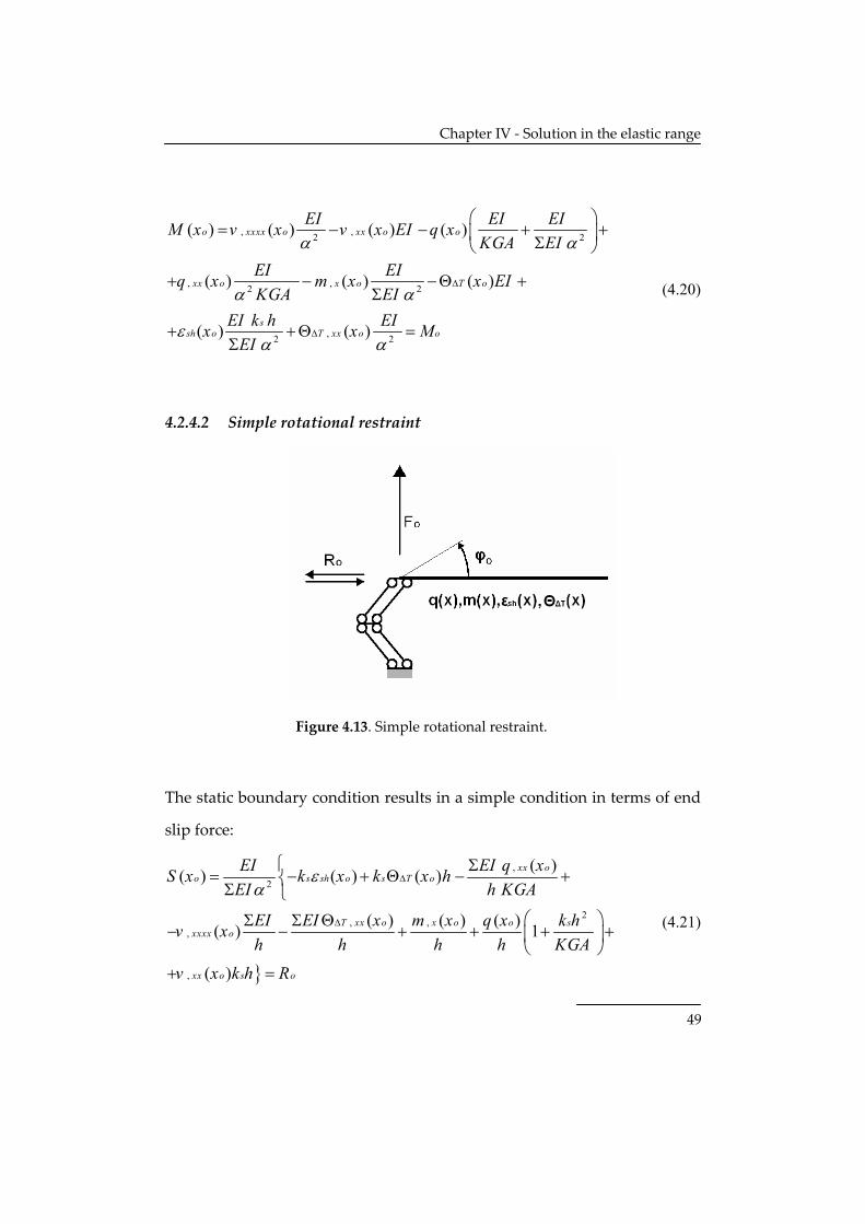
Figure 4.12. Vertical support.
The kinematic boundary condition results in a simple condition in terms of
end transverse displacement:
( )o ov x v= (4.18) The static boundary condition results in a simple condition in terms of end
slip force:
}
,
2
2, ,
,
,
( )( ) ( ) ( )
( ) ( ) ( )( ) 1
( )
xx oo s sh o s T o
T xx o x o o sxxxx o
xx o s o
EI EI q xS x k x k x hEI h KGA
EI EI x m x q x k hv xh h h h KGA
v x k h R
εα
∆
∆
⎧ Σ= − + Θ − +⎨Σ ⎩
⎛ ⎞Σ Σ Θ− − + + + +⎜ ⎟
⎝ ⎠+ =
(4.19)
The second static boundary condition results in a simple condition in terms
of end bending moment:
Page 56
Chapter IV ‐ Solution in the elastic range
49
, ,2 2
, ,2 2
,2 2
( ) ( ) ( ) ( )
( ) ( ) ( )
( ) ( )
o xxxx o xx o o
xx o x o T o
ssh o T xx o o
EI EI EIM x v x v x EI q xKGA EI
EI EIq x m x x EIKGA EI
EI k h EIx x MEI
α α
α α
εα α
∆
∆
⎛ ⎞= − − + +⎜ ⎟Σ⎝ ⎠
+ − −Θ +Σ
+ +Θ =Σ
(4.20)
4.2.4.2 Simple rotational restraint
Figure 4.13. Simple rotational restraint.
The static boundary condition results in a simple condition in terms of end
slip force:
}
,
2
2, ,
,
,
( )( ) ( ) ( )
( ) ( ) ( )( ) 1
( )
xx oo s sh o s T o
T xx o x o o sxxxx o
xx o s o
EI EI q xS x k x k x hEI h KGA
EI EI x m x q x k hv xh h h h KGA
v x k h R
εα
∆
∆
⎧ Σ= − + Θ − +⎨Σ ⎩
⎛ ⎞Σ Σ Θ− − + + + +⎜ ⎟
⎝ ⎠+ =
(4.21)
Page 57
Giuseppe Di Palma 163/000542
50
The kinematic boundary condition results in a simple condition in terms of
end rotational displacement:
( )
, , ,2
, ,
2 2
, , ,
2 2
,
( ) ( ) ( ) ( )
( ) ( ) ( )
( ) ( ) ( )
(
o xxxxx o xxx o x o
x o xxx o o
xx o T x o sh x o s
T xxx
EI EIx v x v x v xKGA KGA
q x EI EI q x EI m xKGA KGA EI KGA KGA KGA
m x EI x x EI k hEIKGA EI KGA KGA EI
x
ϕα
α α
εα α
∆
∆
⎛ ⎞ ⎛ ⎞= − − +⎜ ⎟ ⎜ ⎟⎝ ⎠⎝ ⎠
⎛ ⎞⎛ ⎞− + + + +⎜ ⎟⎜ ⎟Σ⎝ ⎠ ⎝ ⎠Θ⎛ ⎞− − + +⎜ ⎟Σ Σ⎝ ⎠
Θ+ 2
)oo
EIKGA
ϕα
⎛ ⎞ =⎜ ⎟⎝ ⎠
(4.22)
The second static boundary condition results in a simple condition in terms
of end shear stress:
( )
( )
, ,2
, ,2
, , ,2 2 2
,
2
( ) ( ) ( )
( ) ( ) ( )
( ) ( ) ( )
( )
o xxxxx o xxx o
x o T x o o
ssh x o xx o T xxx o
xxx oo
EIQ x v x EI v x
EI EI q x EI x m xKGA EIh k EI EI EIx m x xEI EIEI q x F
KGA
α
α
εα α α
α
∆
∆
⎛ ⎞= − +⎜ ⎟⎝ ⎠
⎡ ⎤− + − Θ + +⎢ ⎥Σ⎣ ⎦⎛ ⎞ ⎛ ⎞ ⎛ ⎞+ − + Θ +⎜ ⎟ ⎜ ⎟ ⎜ ⎟Σ Σ⎝ ⎠ ⎝ ⎠ ⎝ ⎠⎛ ⎞+ =⎜ ⎟⎝ ⎠
(4.23)
Page 58
Chapter IV ‐ Solution in the elastic range
51
4.2.4.3 Mutual horizontal pendulum
Figure 4.14. Mutual horizontal pendulum.
The kinematic boundary condition results in a simple condition in terms of
end slip:
, ,2
,, , ,
,,
1( ) ( ) ( )
( )( ) ( ) ( )
( ) ( )
ss o x o s T x o
s
xx oxxx o s s sh x o T xxx o
xxx oxxxxx o so
EI k hu x q x k h xEI k KGA h
m x EIv x k h k x xh h
EI q x EIv x uh KGA h
α
ε
∆
∆
⎡ ⎛ ⎞= − + + Θ +⎜ ⎟⎢Σ ⎝ ⎠⎣Σ
+ − + − Θ +
Σ Σ ⎤− − =⎥⎦
(4.24)
The static boundary condition results in a simple condition in terms of end
bending moment:
, ,2 2
, ,2 2
,2 2
( ) ( ) ( ) ( )
( ) ( ) ( )
( ) ( )
o xxxx o xx o o
xx o x o T o
ssh o T xx o o
EI EI EIM x v x v x EI q xKGA EI
EI EIq x m x x EIKGA EI
EI k h EIx x MEI
α α
α α
εα α
∆
∆
⎛ ⎞= − − + +⎜ ⎟Σ⎝ ⎠
+ − −Θ +Σ
+ +Θ =Σ
(4.25)
Page 59
Giuseppe Di Palma 163/000542
52
The second static boundary condition results in a simple condition in terms
of end shear stress:
( )
( )
, ,2
, ,2
, , ,2 2 2
,
2
( ) ( ) ( )
( ) ( ) ( )
( ) ( ) ( )
( )
o xxxxx o xxx o
x o T x o o
ssh x o xx o T xxx o
xxx oo
EIQ x v x EI v x
EI EI q x EI x m xKGA EIh k EI EI EIx m x xEI EIEI q x F
KGA
α
α
εα α α
α
∆
∆
⎛ ⎞= − +⎜ ⎟⎝ ⎠
⎡ ⎤− + − Θ + +⎢ ⎥Σ⎣ ⎦⎛ ⎞ ⎛ ⎞ ⎛ ⎞+ − + Θ +⎜ ⎟ ⎜ ⎟ ⎜ ⎟Σ Σ⎝ ⎠ ⎝ ⎠ ⎝ ⎠⎛ ⎞+ =⎜ ⎟⎝ ⎠
(4.26)
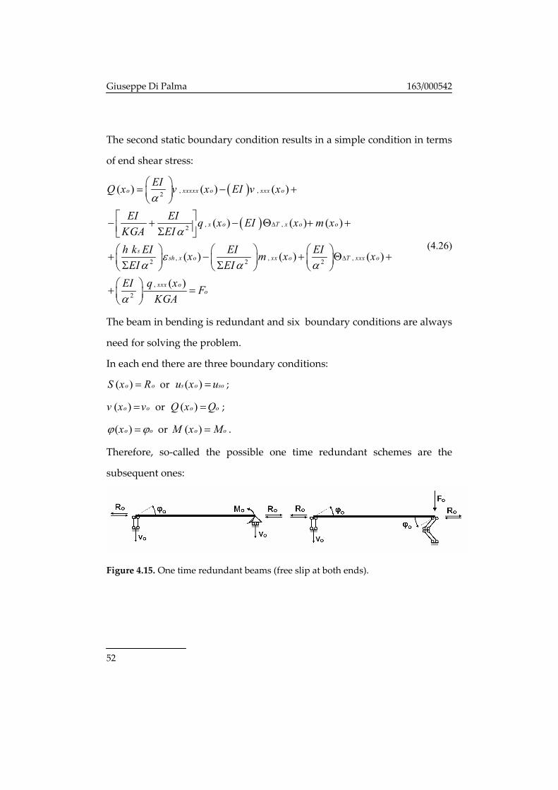
The beam in bending is redundant and six boundary conditions are always
need for solving the problem.
In each end there are three boundary conditions:
( )o oS x R= or ( )s o sou x u= ;
( )o ov x v= or ( )o oQ x Q= ;
( )o oxϕ ϕ= or ( )o oM x M= .
Therefore, so‐called the possible one time redundant schemes are the
subsequent ones:
Figure 4.15. One time redundant beams (free slip at both ends).
Page 60
Chapter IV ‐ Solution in the elastic range
53
Figure 4.16. One time redundant beams (free slip at one end).
Figure 4.17. One time redundant beams (restrained slip at both ends).
The possible two time redundant schemes are the subsequent ones:
Figure 4.18. Two time redundant beam (free slip at both ends).
Page 61
Giuseppe Di Palma 163/000542
54
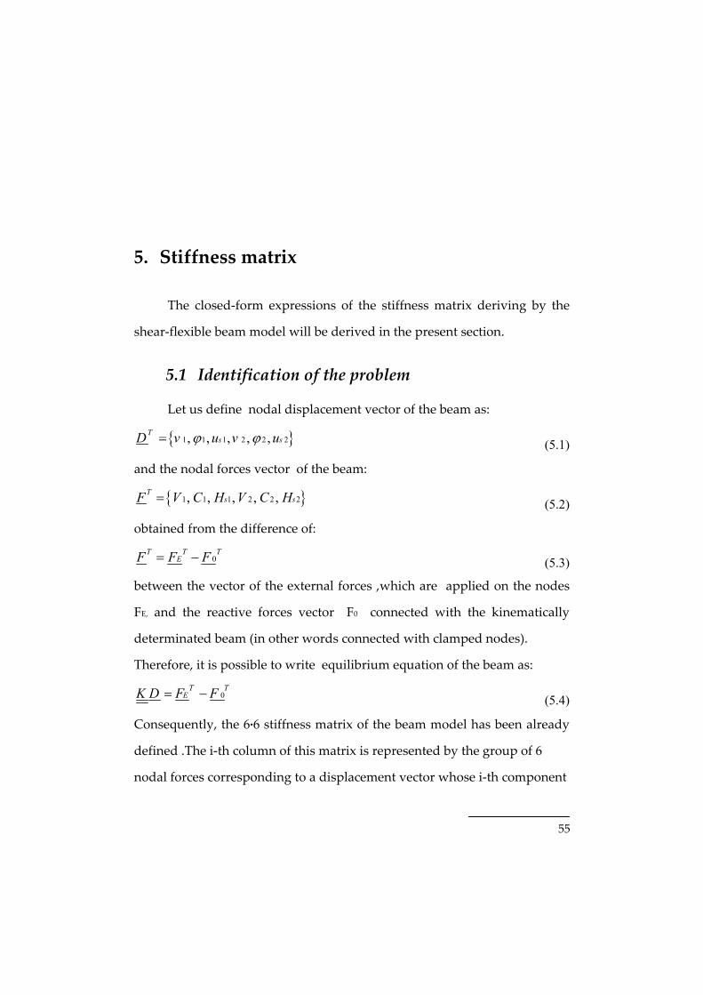
Figure 4.19. Two time redundant beam (free slip at one end).
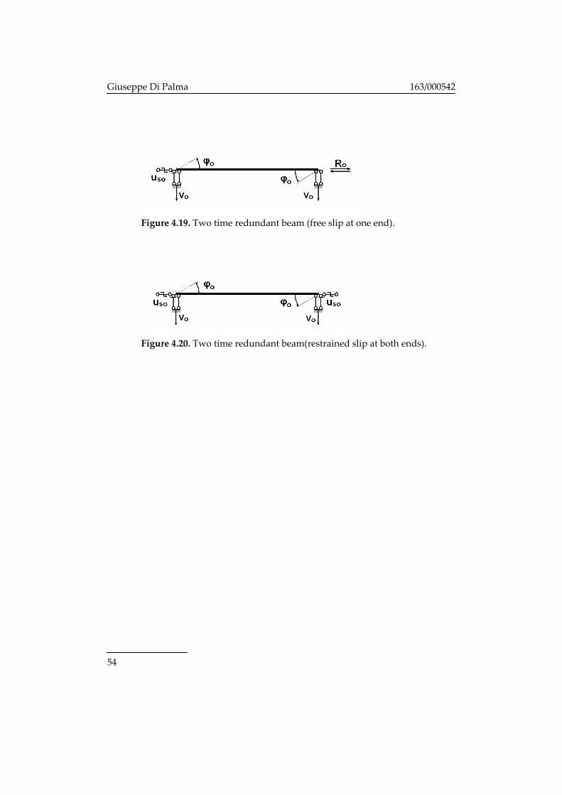
Figure 4.20. Two time redundant beam(restrained slip at both ends).
Page 62
55
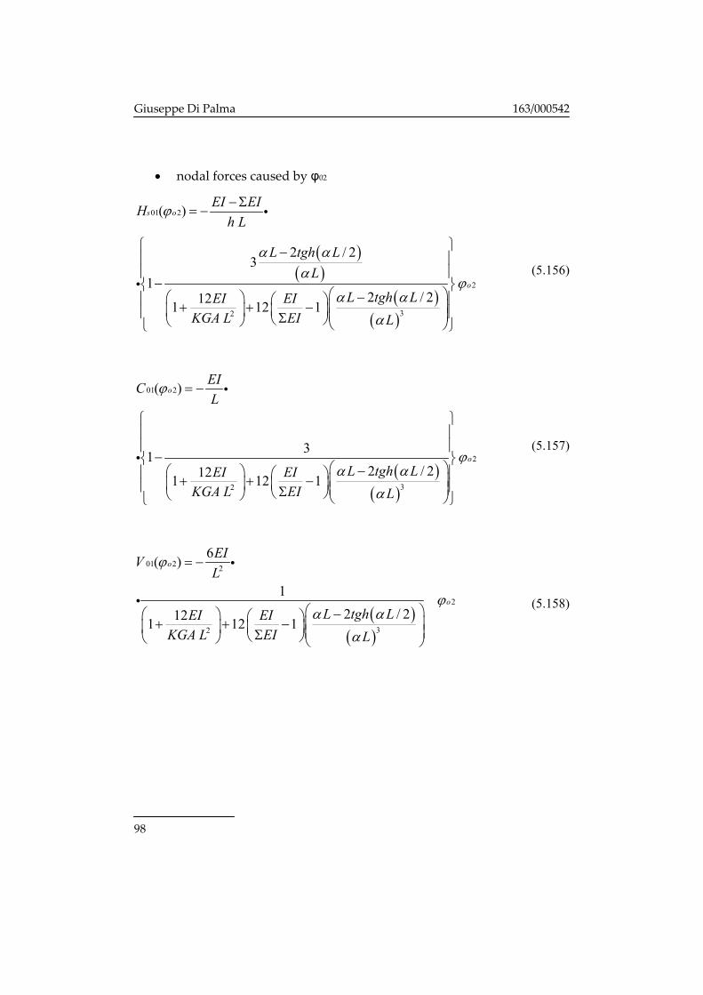
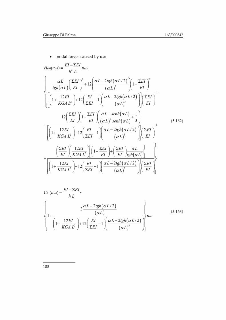
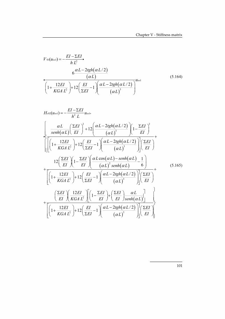
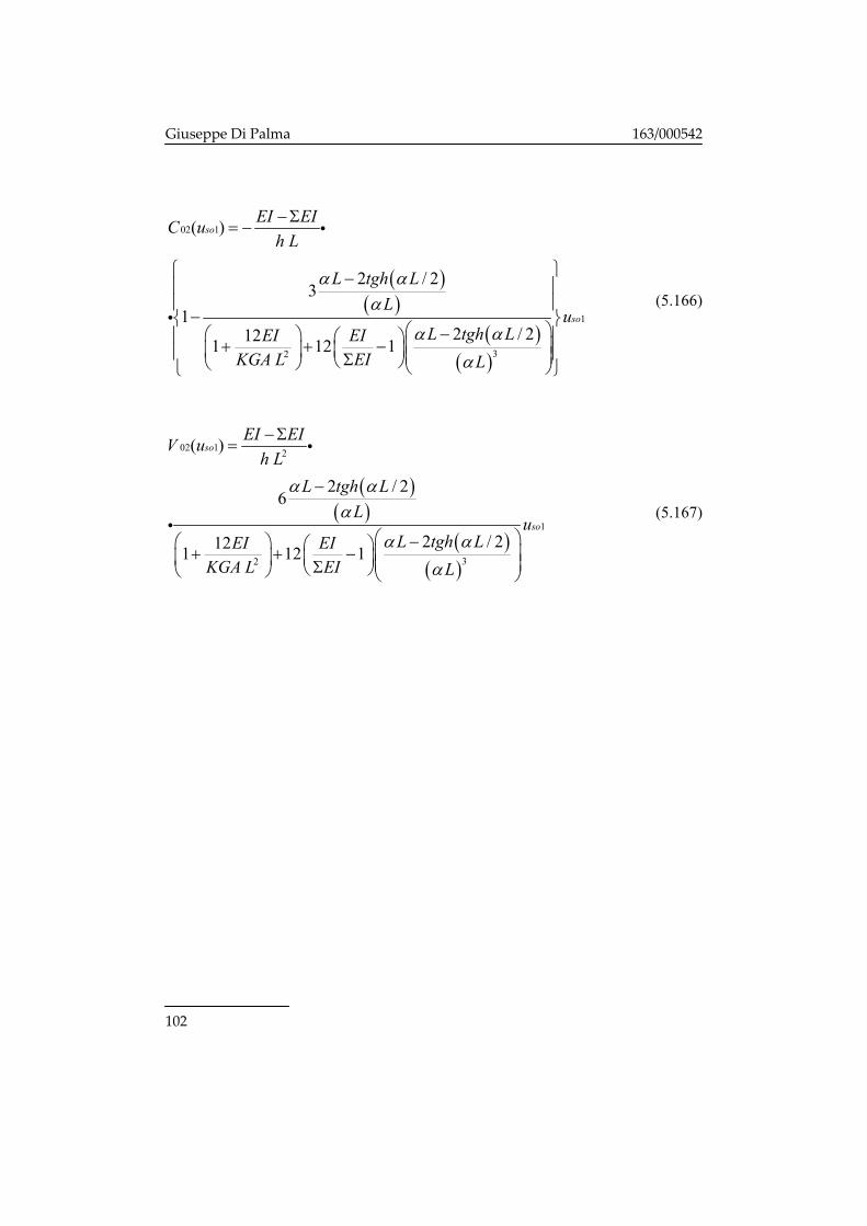
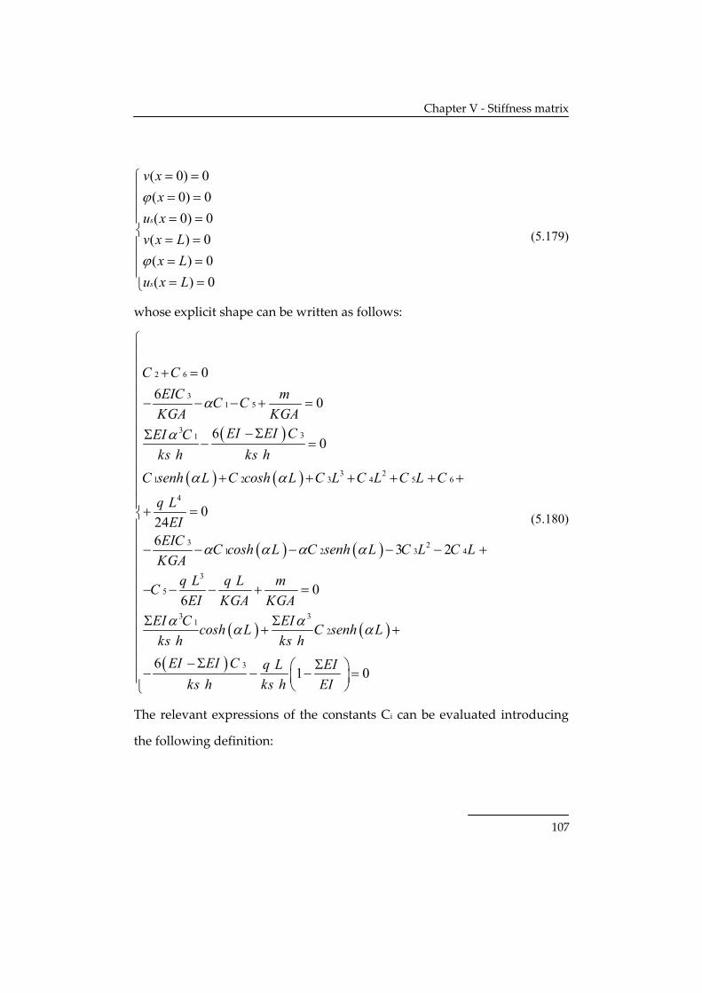
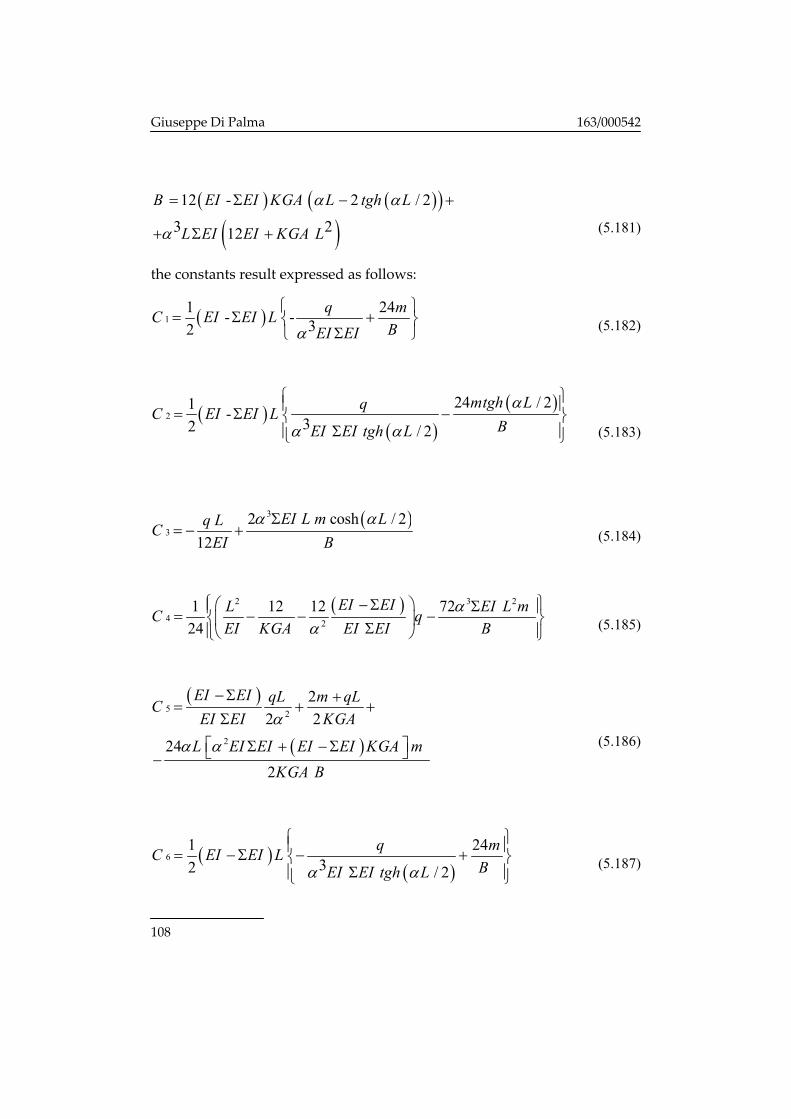
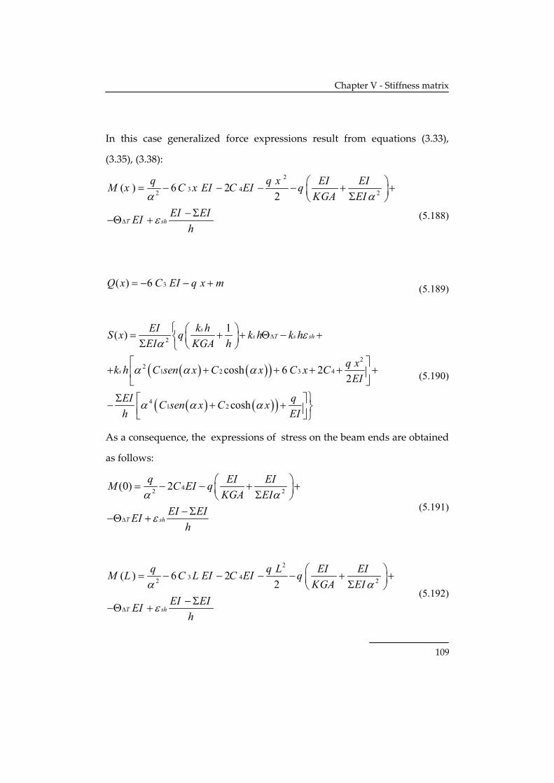
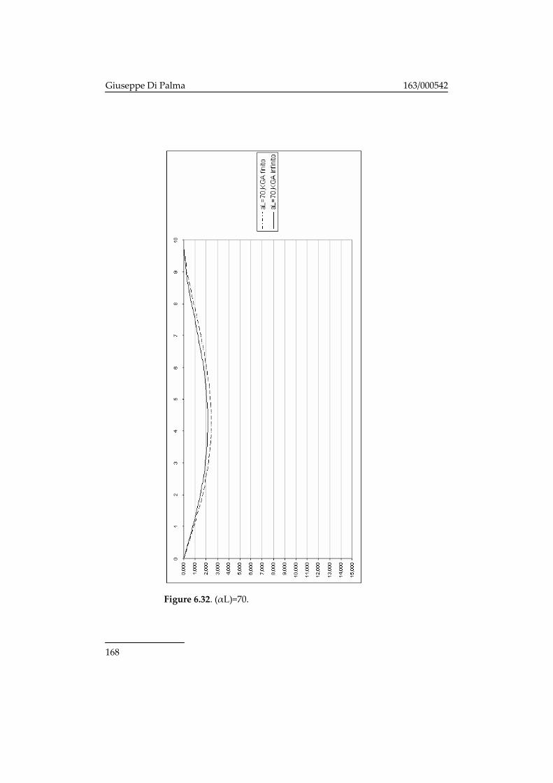
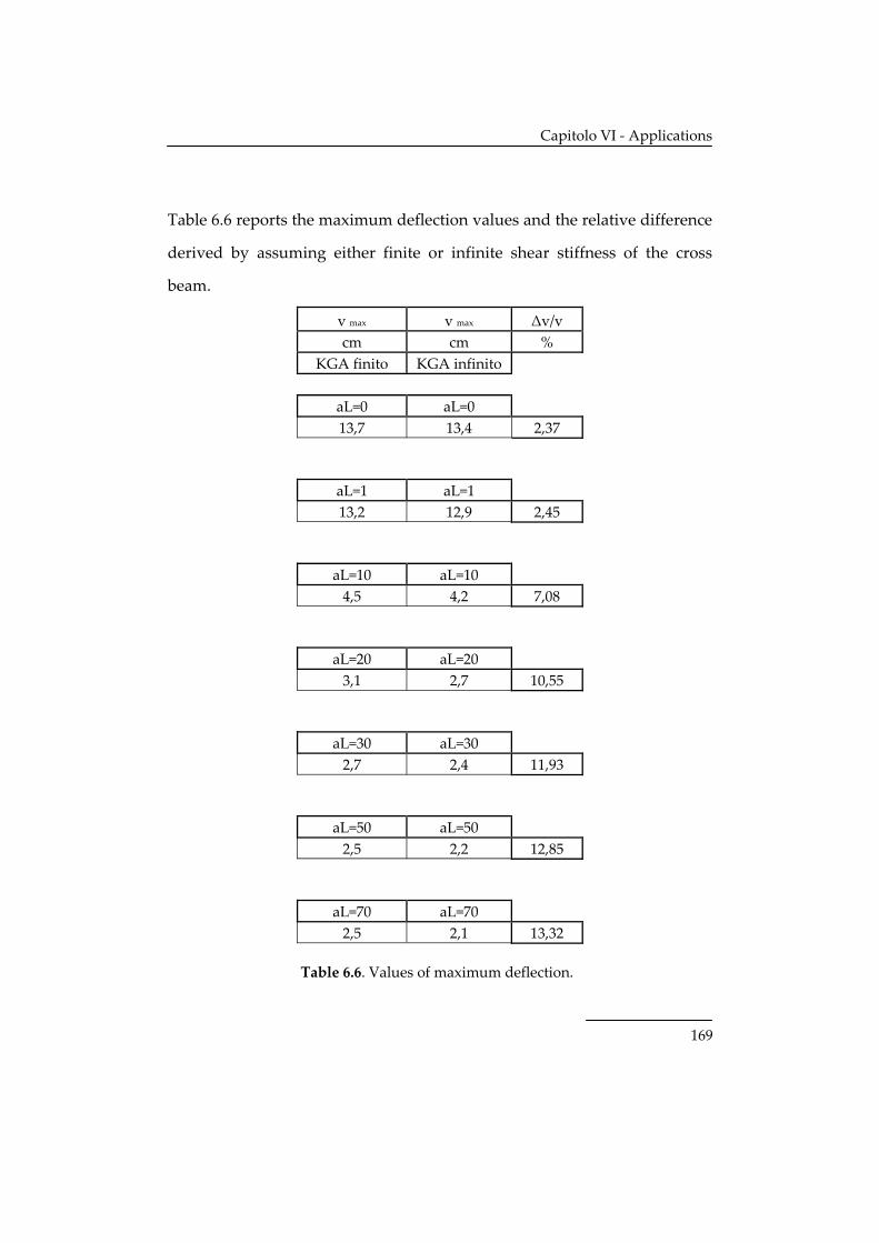
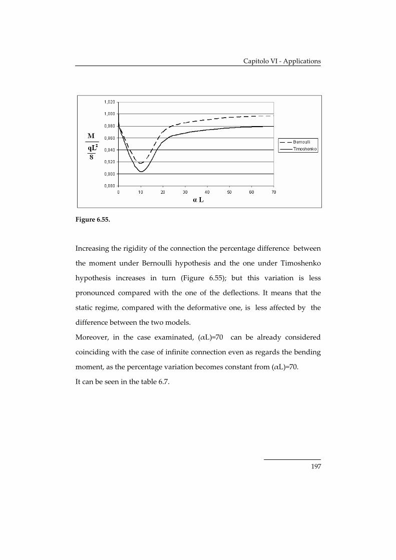
5. Stiffness matrix
The closed‐form expressions of the stiffness matrix deriving by the
shear‐flexible beam model will be derived in the present section.
5.1 Identification of the problem
Let us define nodal displacement vector of the beam as:
{ }1 1 1 2 2 2, , , , ,Ts sD v u v uϕ ϕ= (5.1)
and the nodal forces vector of the beam:
{ }1 1 1 2 2 2, , , , ,Ts sF V C H V C H= (5.2)
obtained from the difference of:
0T T T
EF F F= − (5.3)
between the vector of the external forces ,which are applied on the nodes
FE, and the reactive forces vector F0 connected with the kinematically
determinated beam (in other words connected with clamped nodes).
Therefore, it is possible to write equilibrium equation of the beam as:
0T TEK D F F= − (5.4)
Consequently, the 6∙6 stiffness matrix of the beam model has been already
defined .The i‐th column of this matrix is represented by the group of 6
nodal forces corresponding to a displacement vector whose i‐th component
Page 63
Giuseppe Di Palma 163/000542
56
is one and the other zero.
Displacements and nodal forces which are both dual with each other, have
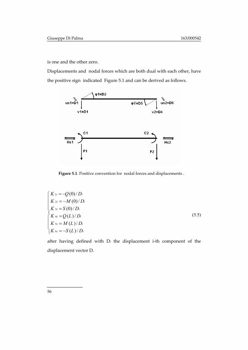
the positive sign indicated Figure 5.1 and can be derived as follows.
Figure 5.1. Positive convention for nodal forces and displacements .
1
2
3
4
5
6
(0) /(0) /
(0) /( ) /( ) /( ) /
i i
i i
i i
i i
i i
i i
K Q DK M DK S DK Q L DK M L DK S L D
= −⎧⎪ = −⎪⎪ =⎨ =⎪⎪ =⎪
= −⎩
(5.5)
after having defined with Di the displacement i‐th component of the
displacement vector D.
Page 64
Chapter V ‐ Stiffness matrix
57
5.2 Coefficients of the stiffness matrix
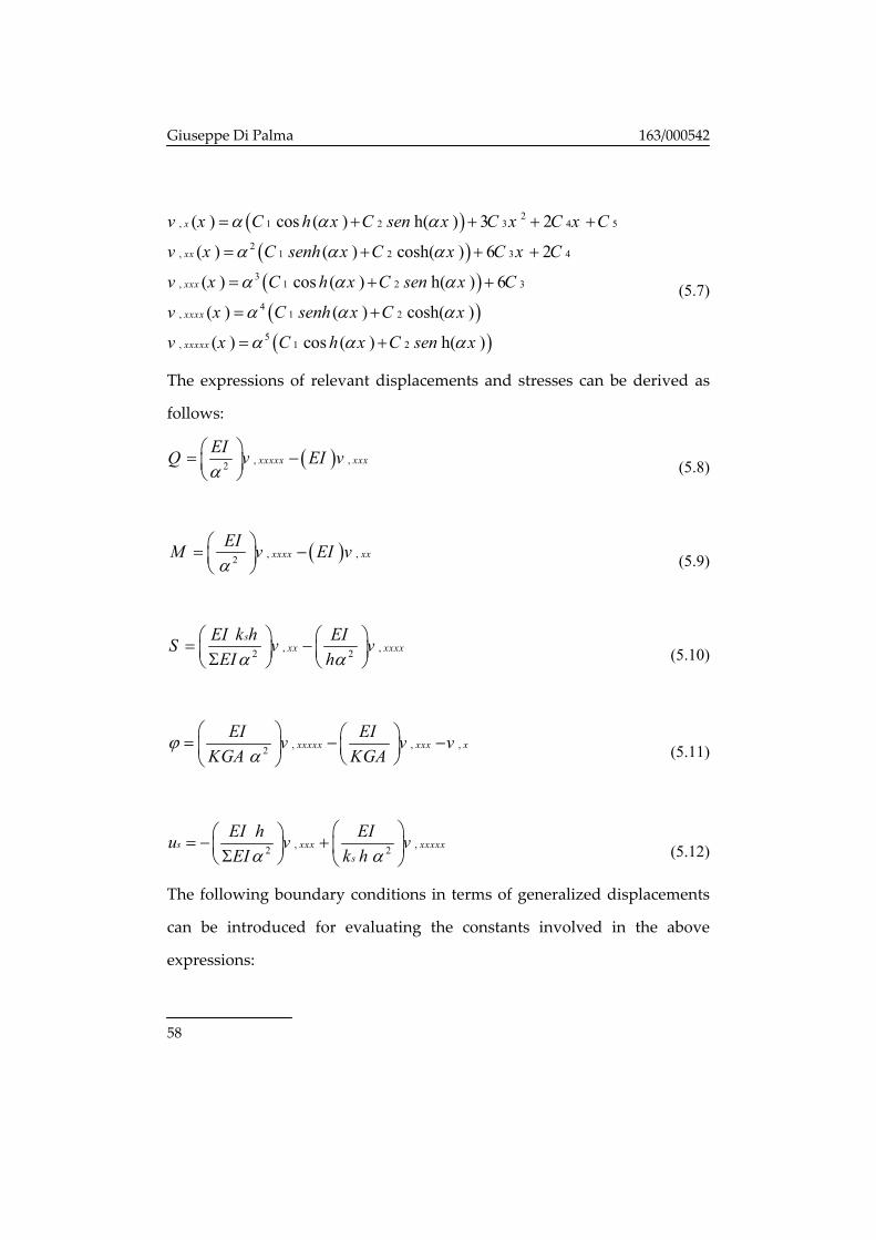
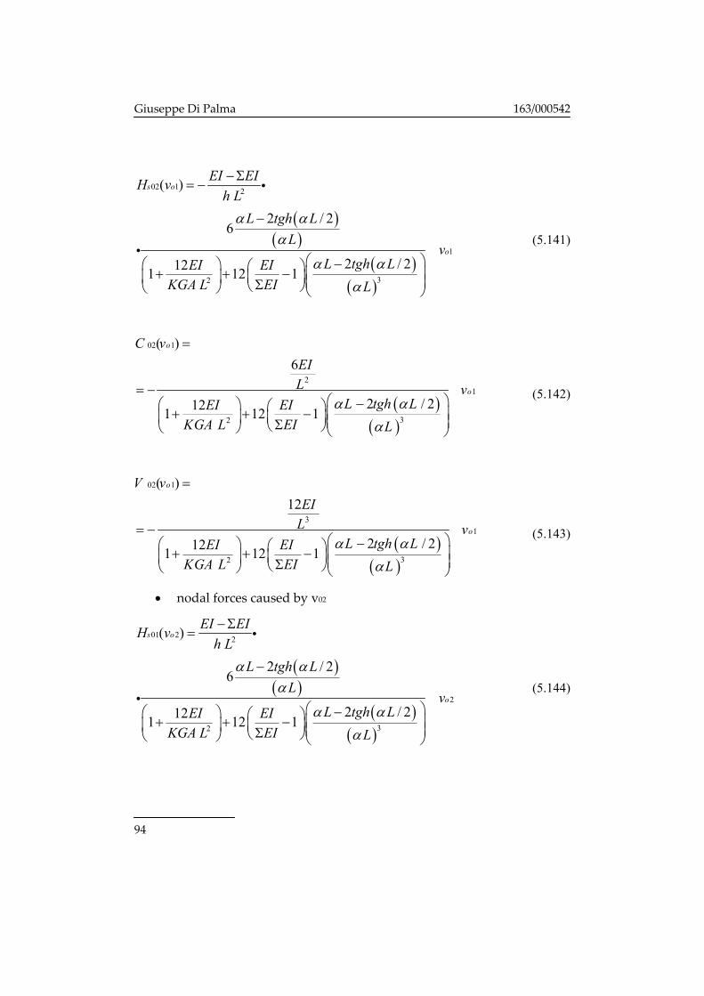
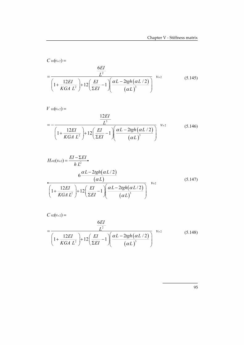
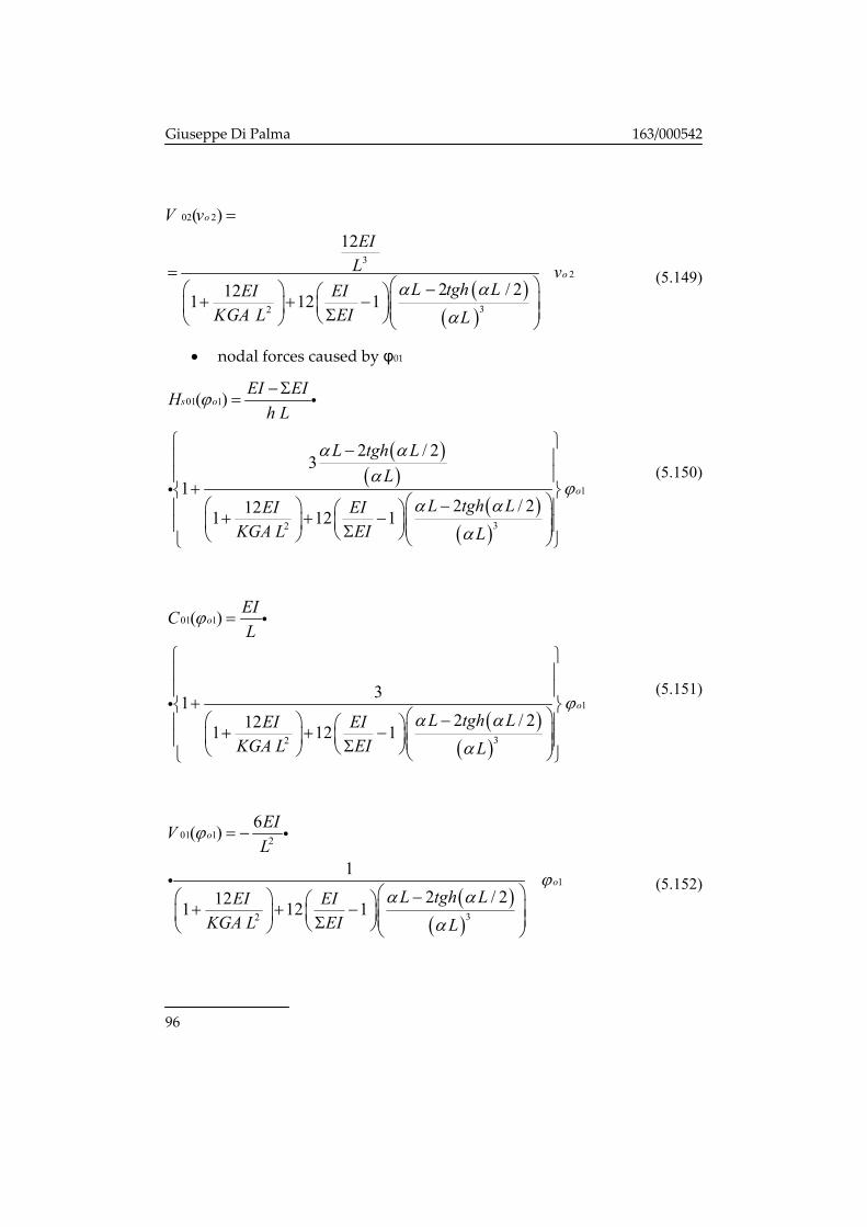
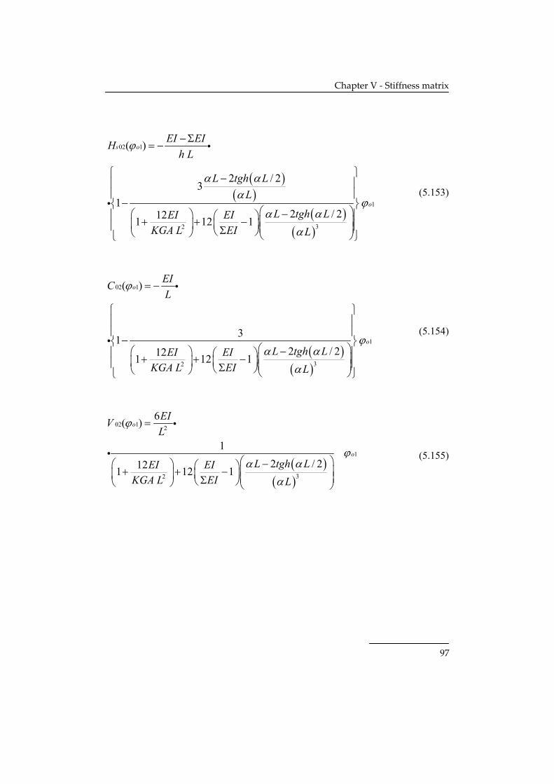
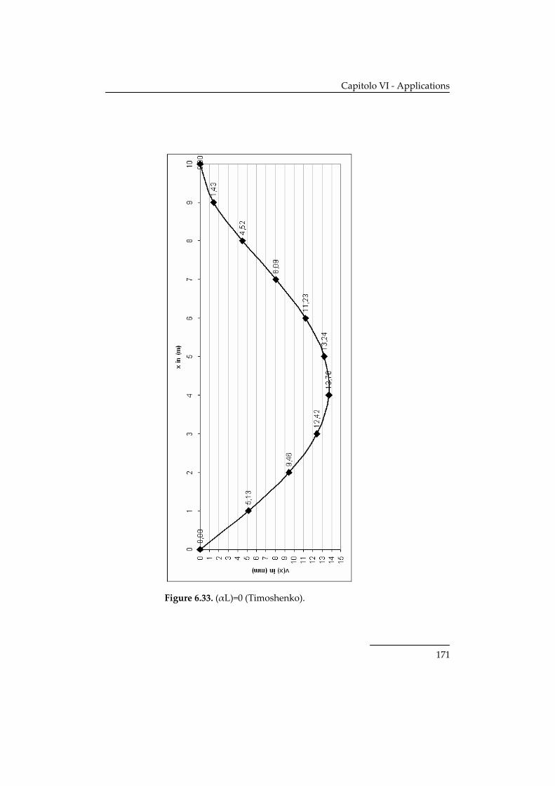
5.2.1 General procedure for deriving the integration constants
The term of the stiffness matrix can be derived by solving the
differential equation imposing nodal displacements in each component as
the others are forced to zero.
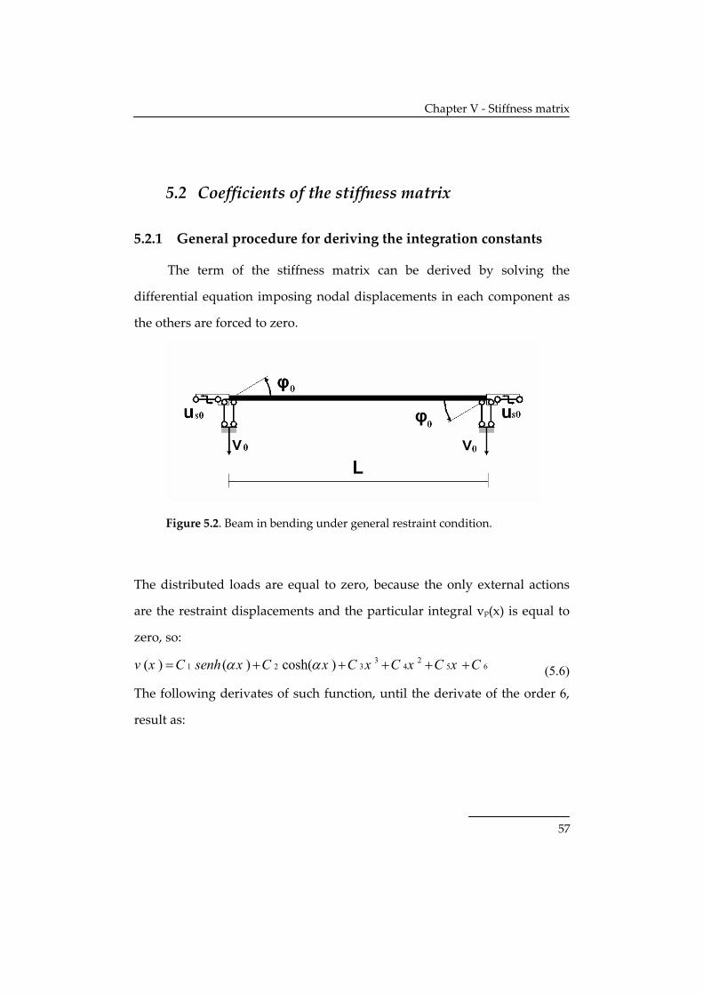
Figure 5.2. Beam in bending under general restraint condition.
The distributed loads are equal to zero, because the only external actions
are the restraint displacements and the particular integral vp(x) is equal to
zero, so: 3 2
1 2 3 4 5 6( ) ( ) cosh( )v x C senh x C x C x C x C x Cα α= + + + + + (5.6)
The following derivates of such function, until the derivate of the order 6,
result as:
Page 65
Giuseppe Di Palma 163/000542
58
( )( )( )( )( )
2, 1 2 3 4 5
2, 1 2 3 4
3, 1 2 3
4, 1 2
5, 1 2
( ) cos ( ) h( ) 3 2
( ) ( ) cosh( ) 6 2
( ) cos ( ) h( ) 6
( ) ( ) cosh( )
( ) cos ( ) h( )
x
xx
xxx
xxxx
xxxxx
v x C h x C sen x C x C x C
v x C senh x C x C x C
v x C h x C sen x C
v x C senh x C x
v x C h x C sen x
α α α
α α α
α α α
α α α
α α α
= + + + +
= + + +
= + +
= +
= +
(5.7)
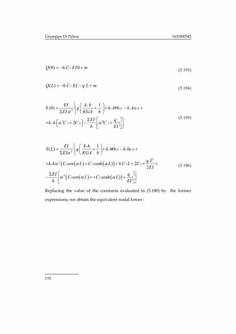
The expressions of relevant displacements and stresses can be derived as
follows:
( ), ,2 xxxxx xxxEIQ v EI vα⎛ ⎞= −⎜ ⎟⎝ ⎠
(5.8)
( ), ,2 xxxx xxEIM v EI vα
⎛ ⎞= −⎜ ⎟⎝ ⎠
(5.9)
, ,2 2
sxx xxxx
EI k h EIS v vEI hα α
⎛ ⎞ ⎛ ⎞= −⎜ ⎟ ⎜ ⎟Σ⎝ ⎠ ⎝ ⎠ (5.10)
, , ,2 xxxxx xxx xEI EIv v v
KGA KGAϕ
α⎛ ⎞ ⎛ ⎞= − −⎜ ⎟ ⎜ ⎟
⎝ ⎠⎝ ⎠ (5.11)
, ,2 2s xxx xxxxxs
EI h EIu v vEI k hα α
⎛ ⎞⎛ ⎞= − + ⎜ ⎟⎜ ⎟Σ⎝ ⎠ ⎝ ⎠ (5.12)
The following boundary conditions in terms of generalized displacements
can be introduced for evaluating the constants involved in the above
expressions:
Page 66
Chapter V ‐ Stiffness matrix
59
1
1
1
2
2
2
( 0)( 0)( 0)
( )( )( )
s s
s s
v x vx
u x uv x L vx L
u x L u
ϕ ϕ
ϕ ϕ
= =⎧⎪ = =⎪⎪ = =⎨ = =⎪⎪ = =⎪
= =⎩
(5.13)
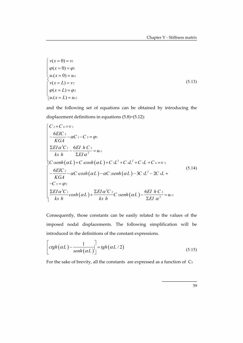
and the following set of equations can be obtained by introducing the
displacement definitions in equations (5.8)÷(5.12):
( ) ( )
( ) ( )
( ) ( )
2 6 1
31 5 1
31 3
12
3 21 2 3 4 5 6 2
3 21 2 3 4
5 2
3 31 2 3
2 22
6
6
6 3 2
6
s
s
C C vEIC C CKGAEI C EI h C uks h EI
C senh L C cosh L C L C L C L C vEIC C cosh L C senh L C L C LKGACEI C EI C EI h Ccosh L C senh L uks h ks h EI
α ϕ
αα
α α
α α α α
ϕ
α αα αα
+ =⎧⎪⎪− − − =⎪⎪Σ⎪ − =
Σ⎪⎪ + + + + + =⎨⎪⎪− − − − − +
− =
Σ Σ+ − =
Σ⎩
⎪⎪⎪⎪⎪
(5.14)
Consequently, those constants can be easily related to the values of the
imposed nodal displacements. The following simplification will be
introduced in the definitions of the constant expressions.
( ) ( ) ( )1 / 2ctgh L tgh Lsenh L
α αα
⎡ ⎤− =⎢ ⎥
⎣ ⎦ (5.15)
For the sake of brevity, all the constants are expressed as a function of C3.
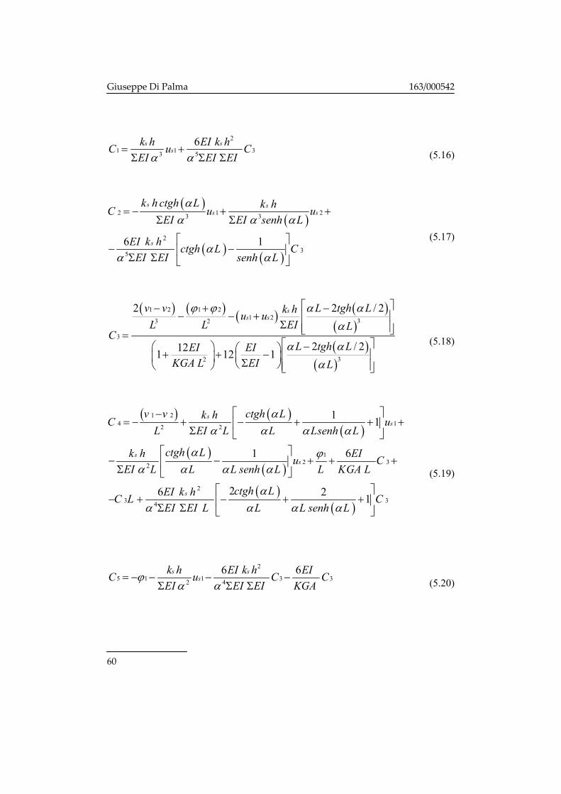
Page 67
Giuseppe Di Palma 163/000542
60
2
1 1 33 5
6s ss
k h EI k hC u CEI EI EIα α
= +Σ Σ Σ
(5.16)
( )( )
( ) ( )
2 1 23 3
2
35
6 1
s ss s
s
k h ctgh L k hC u uEI EI senh L
EI k h ctgh L CEI EI senh L
αα α α
αα α
= − + +Σ Σ
⎡ ⎤− −⎢ ⎥Σ Σ ⎣ ⎦
(5.17)
( ) ( ) ( ) ( )( )( )
( )
1 2 1 21 2 33 2
3
32
2 2 / 2
2 / 2121 12 1
ss s
v v L tgh Lk hu uL L EI L
CL tgh LEI EI
KGA L EI L
ϕ ϕ α αα
α αα
⎡ ⎤− + −− − + ⎢ ⎥
Σ ⎢ ⎥⎣ ⎦=⎡ ⎤−⎛ ⎞ ⎛ ⎞+ + − ⎢ ⎥⎜ ⎟⎜ ⎟ Σ⎝ ⎠⎝ ⎠ ⎢ ⎥⎣ ⎦
(5.18)
( ) ( )( )
( )( )
( )( )
1 24 12 2
12 32
2
3 34
1 1
1 6
26 2 1
ss
ss
s
v v ctgh Lk hC uL EI L L Lsenh L
ctgh Lk h EIu CEI L L L senh L L KGA L
ctgh LEI k hC L CEI EI L L L senh L
αα α α α
α ϕα α α α
αα α α α
⎡ ⎤−= − + − + + +⎢ ⎥Σ ⎣ ⎦
⎡ ⎤− − + + +⎢ ⎥Σ ⎣ ⎦
⎡ ⎤− + − + +⎢ ⎥Σ Σ ⎣ ⎦
(5.19)
2
5 1 1 3 32 4
6 6s ss
k h EI k h EIC u C CEI EI EI KGA
ϕα α
= − − − −Σ Σ Σ
(5.20)
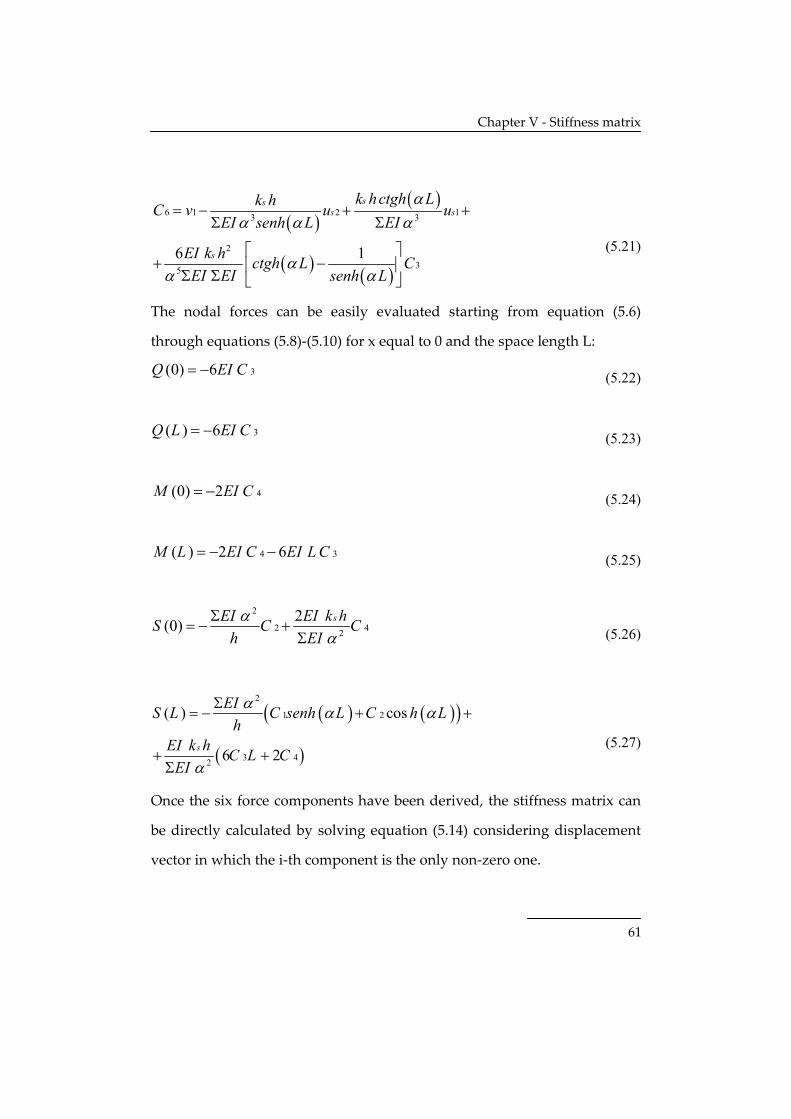
Page 68
Chapter V ‐ Stiffness matrix
61
( )( )
( ) ( )
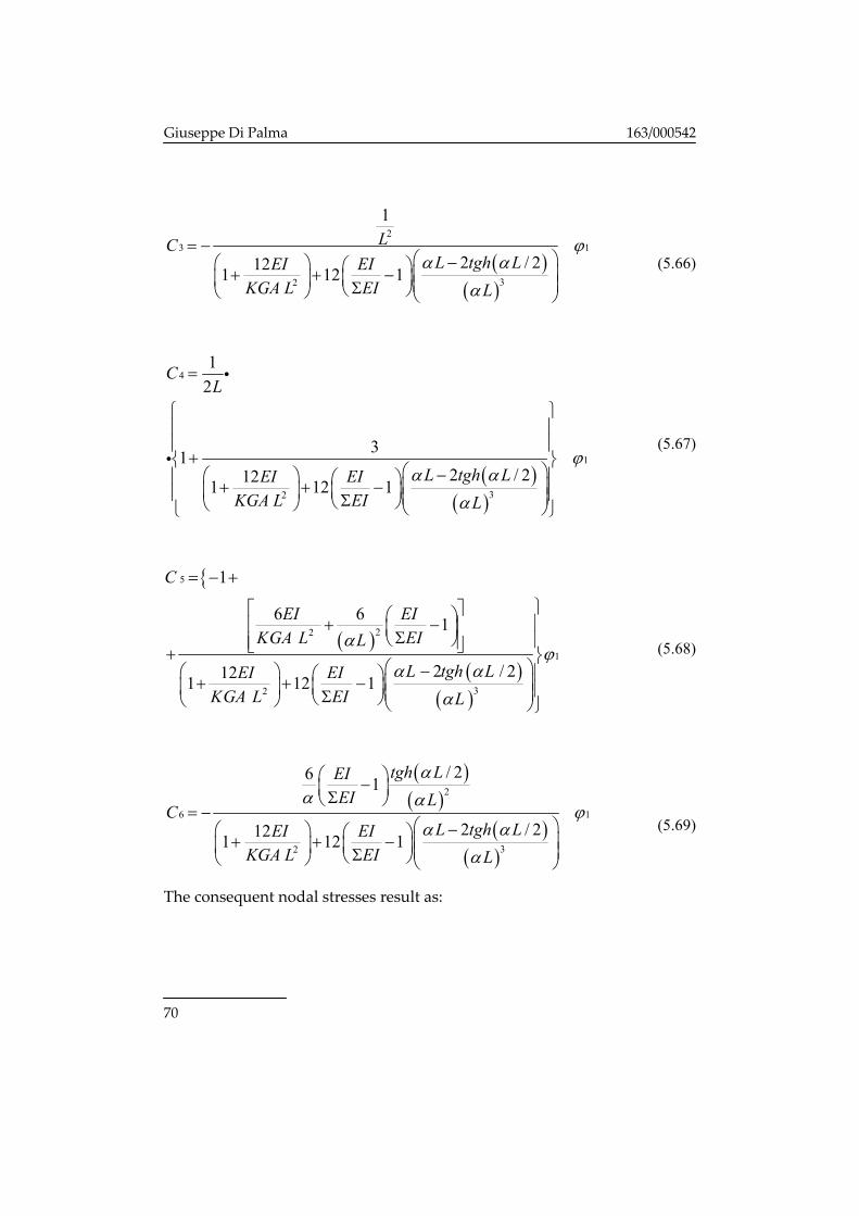
6 1 2 13 3
2
35
6 1
sss s
s
k hctgh Lk hC v u uEI senh L EI
EI k h ctgh L CEI EI senh L
αα α α
αα α
= − + +Σ Σ
⎡ ⎤+ −⎢ ⎥Σ Σ ⎣ ⎦
(5.21)
The nodal forces can be easily evaluated starting from equation (5.6)
through equations (5.8)‐(5.10) for x equal to 0 and the space length L:
3(0) 6Q EI C= − (5.22)
3( ) 6Q L EI C= − (5.23)
4(0) 2M EI C= − (5.24)
4 3( ) 2 6M L EI C EI LC= − − (5.25)
2
2 42
2(0) sEI EI k hS C Ch EIα
αΣ
= − +Σ
(5.26)
( ) ( )( )
( )
2
1 2
3 42
( ) cos
6 2s
EIS L C senh L C h Lh
EI k h C L CEI
α α α
α
Σ= − + +
+ +Σ
(5.27)
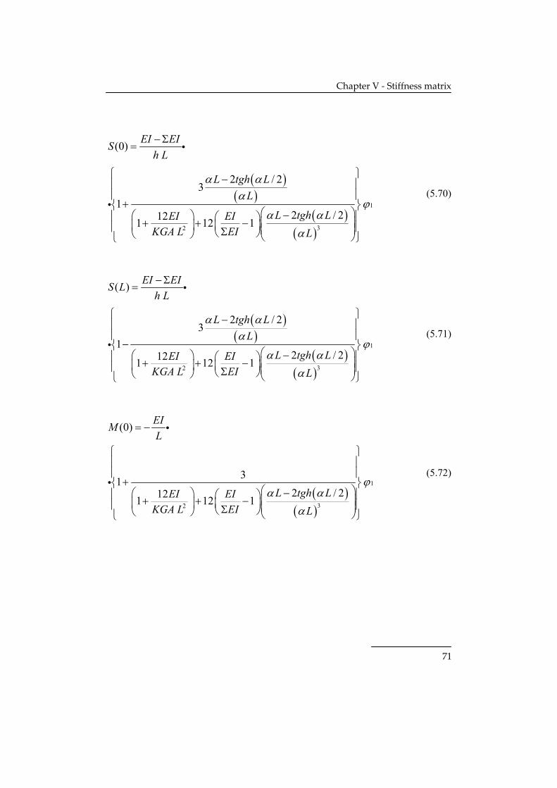
Once the six force components have been derived, the stiffness matrix can
be directly calculated by solving equation (5.14) considering displacement
vector in which the i‐th component is the only non‐zero one.
Page 69
Giuseppe Di Palma 163/000542
62
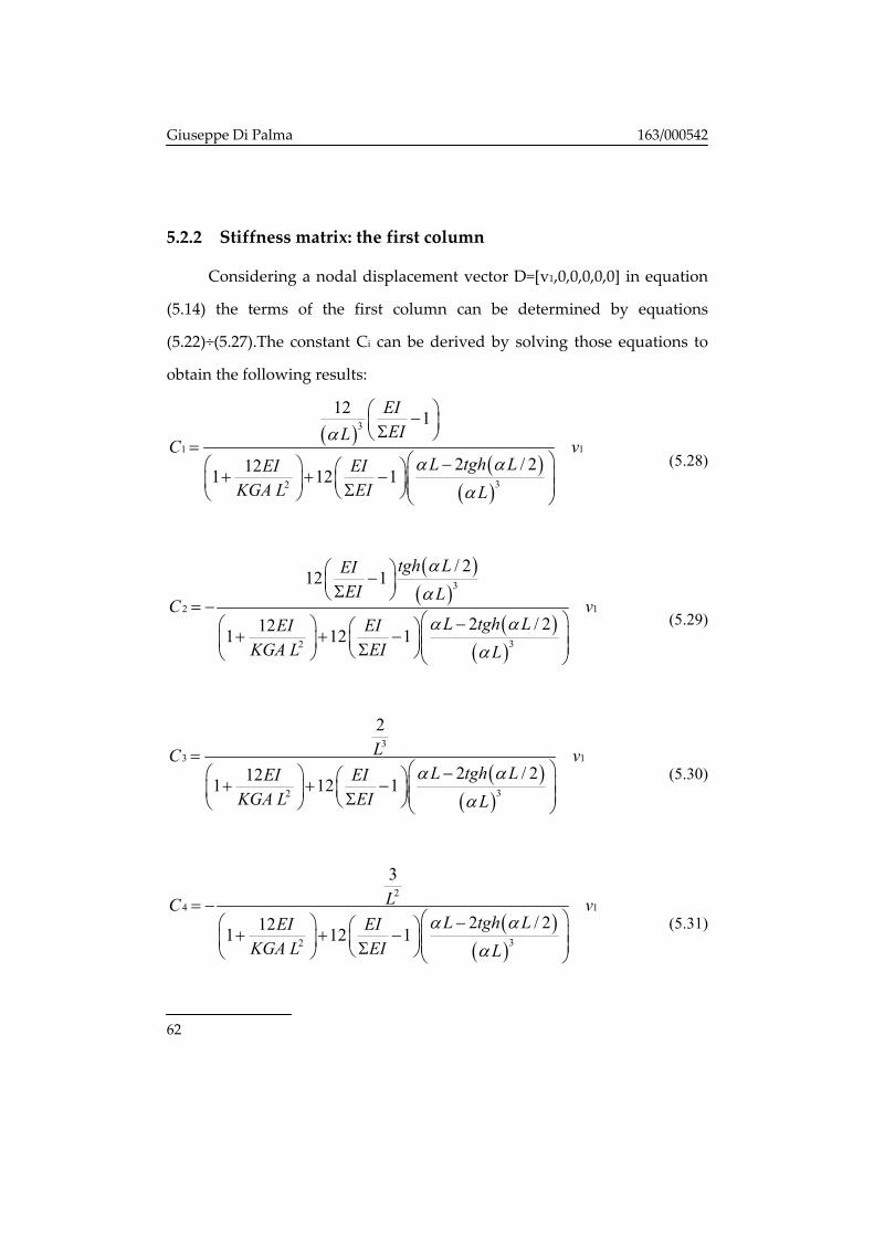
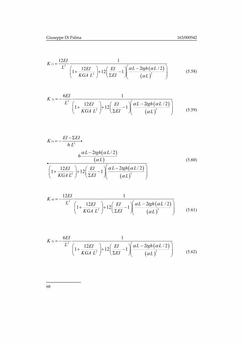
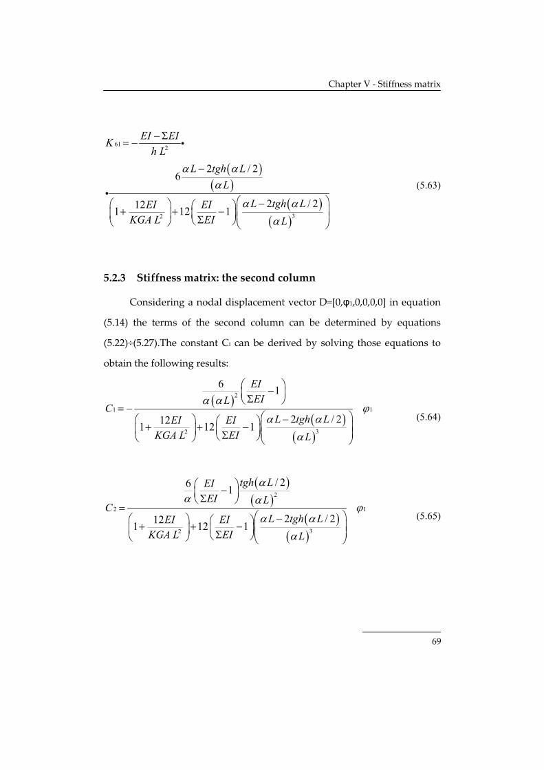
5.2.2 Stiffness matrix: the first column
Considering a nodal displacement vector D=[v1,0,0,0,0,0] in equation
(5.14) the terms of the first column can be determined by equations
(5.22)÷(5.27).The constant Ci can be derived by solving those equations to
obtain the following results:
( )( )
( )
3
1 1
32
12 1
2 / 2121 12 1
EIEIL
C vL tgh LEI EI
KGA L EI L
α
α αα
⎛ ⎞−⎜ ⎟Σ⎝ ⎠=
⎛ ⎞−⎛ ⎞ ⎛ ⎞+ + − ⎜ ⎟⎜ ⎟⎜ ⎟ ⎜ ⎟Σ⎝ ⎠⎝ ⎠ ⎝ ⎠
(5.28)
( )( )
( )( )
3
2 1
32
/ 212 1
2 / 2121 12 1
tgh LEIEI L
C vL tgh LEI EI
KGA L EI L
αα
α αα
⎛ ⎞−⎜ ⎟Σ⎝ ⎠= −
⎛ ⎞−⎛ ⎞ ⎛ ⎞+ + − ⎜ ⎟⎜ ⎟⎜ ⎟ ⎜ ⎟Σ⎝ ⎠⎝ ⎠ ⎝ ⎠
(5.29)
( )( )
33 1
32
2
2 / 2121 12 1
LC vL tgh LEI EI
KGA L EI Lα α
α
=⎛ ⎞−⎛ ⎞ ⎛ ⎞+ + − ⎜ ⎟⎜ ⎟⎜ ⎟ ⎜ ⎟Σ⎝ ⎠⎝ ⎠ ⎝ ⎠
(5.30)
( )( )
24 1
32
3
2 / 2121 12 1
LC vL tgh LEI EI
KGA L EI Lα α
α
= −⎛ ⎞−⎛ ⎞ ⎛ ⎞+ + − ⎜ ⎟⎜ ⎟⎜ ⎟ ⎜ ⎟Σ⎝ ⎠⎝ ⎠ ⎝ ⎠
(5.31)
Page 70
Chapter V ‐ Stiffness matrix
63
( )( )
3 2
5 1
32
12 1 1
2 / 2121 12 1
EI EIL KGA EIC v
L tgh LEI EIKGA L EI L
α
α αα
⎡ ⎤⎛ ⎞+ −⎜ ⎟⎢ ⎥Σ⎝ ⎠⎣ ⎦= −⎛ ⎞−⎛ ⎞ ⎛ ⎞+ + − ⎜ ⎟⎜ ⎟⎜ ⎟ ⎜ ⎟Σ⎝ ⎠⎝ ⎠ ⎝ ⎠
(5.32)
( )( )
( )( )
3
6 1
32
/ 212 1
12 / 2121 12 1
tgh LEIEI L
C vL tgh LEI EI
KGA L EI L
αα
α αα
⎧ ⎫⎛ ⎞⎪ ⎪−⎜ ⎟Σ⎪ ⎪⎝ ⎠= +⎨ ⎬
⎛ ⎞−⎛ ⎞⎪ ⎪⎛ ⎞+ + − ⎜ ⎟⎜ ⎟⎜ ⎟⎪ ⎪⎜ ⎟Σ⎝ ⎠⎝ ⎠ ⎝ ⎠⎩ ⎭
(5.33)
Hence, the following nodal forces can be derived:
( )( )
( )( )
2
1
32
(0)
2 / 26
2 / 2121 12 1
EI EISh L
L tgh LL
vL tgh LEI EI
KGA L EI L
α αα
α αα
−Σ= −
−
⎛ ⎞−⎛ ⎞ ⎛ ⎞+ + − ⎜ ⎟⎜ ⎟⎜ ⎟ ⎜ ⎟Σ⎝ ⎠⎝ ⎠ ⎝ ⎠
i
i (5.34)
( )( )
( )( )
2
1
32
( )
2 / 26
2 / 2121 12 1
EI EIS Lh L
L tgh LL
vL tgh LEI EI
KGA L EI L
α αα
α αα
−Σ=
−
⎛ ⎞−⎛ ⎞ ⎛ ⎞+ + − ⎜ ⎟⎜ ⎟⎜ ⎟ ⎜ ⎟Σ⎝ ⎠⎝ ⎠ ⎝ ⎠
i
i (5.35)
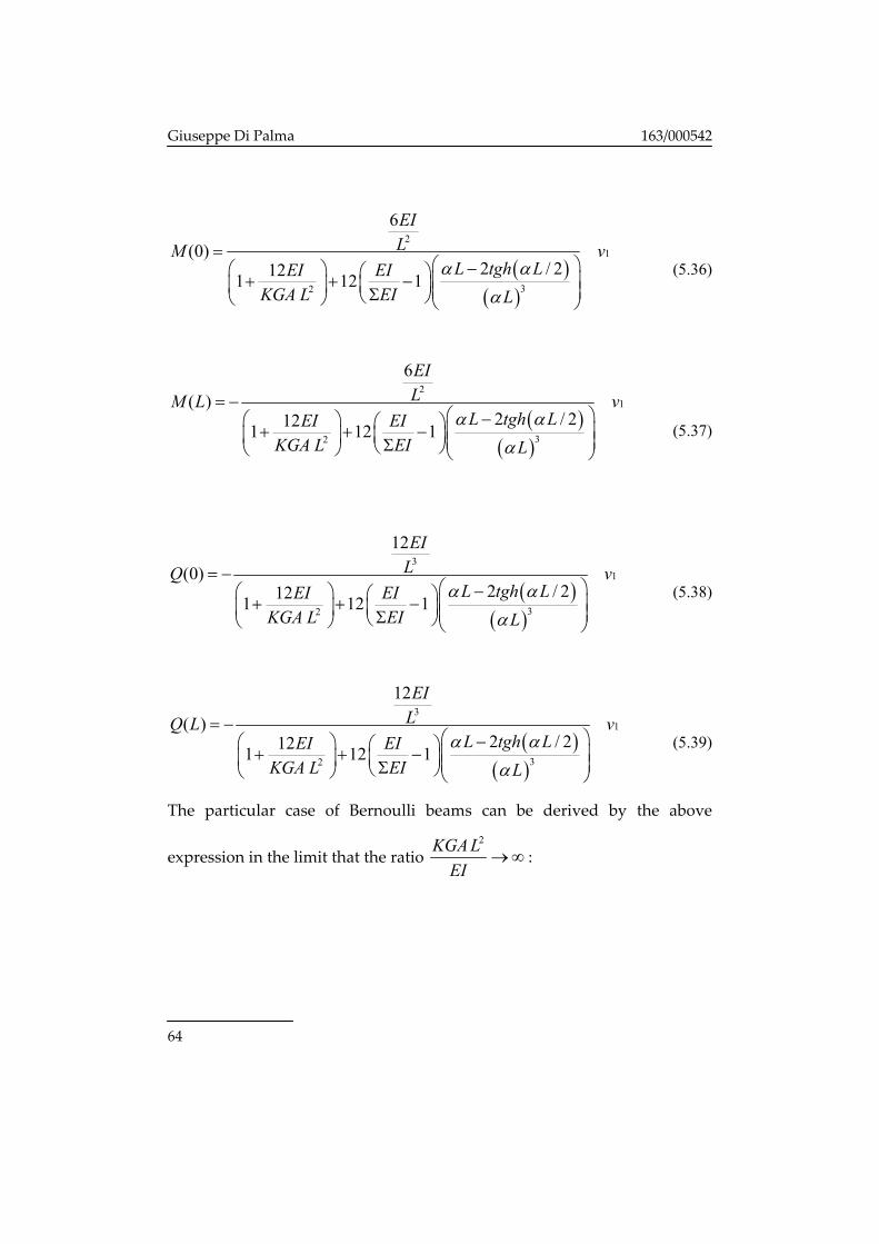
Page 71
Giuseppe Di Palma 163/000542
64
( )( )
21
32
6
(0)2 / 2121 12 1
EILM v
L tgh LEI EIKGA L EI L
α αα
=⎛ ⎞−⎛ ⎞ ⎛ ⎞+ + − ⎜ ⎟⎜ ⎟⎜ ⎟ ⎜ ⎟Σ⎝ ⎠⎝ ⎠ ⎝ ⎠
(5.36)
( )( )
21
32
6
( )2 / 2121 12 1
EILM L v
L tgh LEI EIKGA L EI L
α αα
= −⎛ ⎞−⎛ ⎞ ⎛ ⎞+ + − ⎜ ⎟⎜ ⎟⎜ ⎟ ⎜ ⎟Σ⎝ ⎠⎝ ⎠ ⎝ ⎠
(5.37)
( )( )
31
32
12
(0)2 / 2121 12 1
EILQ v
L tgh LEI EIKGA L EI L
α αα
= −⎛ ⎞−⎛ ⎞ ⎛ ⎞+ + − ⎜ ⎟⎜ ⎟⎜ ⎟ ⎜ ⎟Σ⎝ ⎠⎝ ⎠ ⎝ ⎠
(5.38)
( )( )
31
32
12
( )2 / 2121 12 1
EILQ L v
L tgh LEI EIKGA L EI L
α αα
= −⎛ ⎞−⎛ ⎞ ⎛ ⎞+ + − ⎜ ⎟⎜ ⎟⎜ ⎟ ⎜ ⎟Σ⎝ ⎠⎝ ⎠ ⎝ ⎠
(5.39)
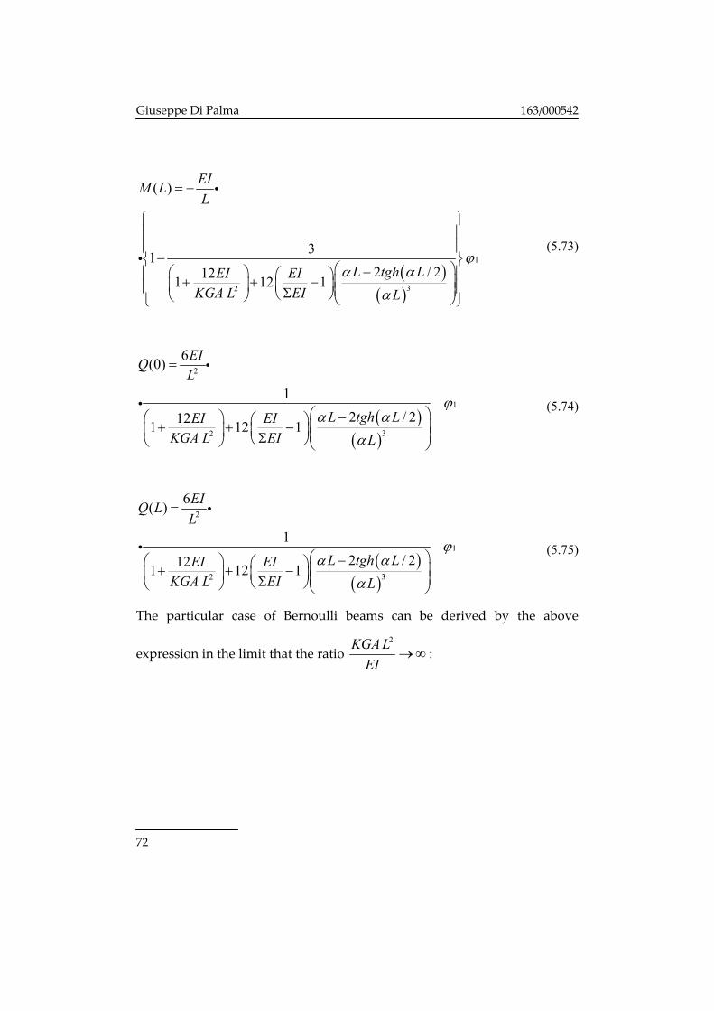
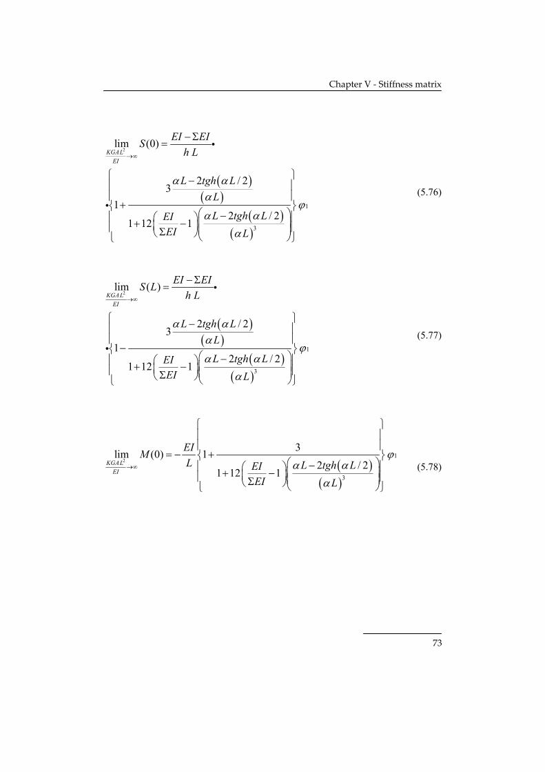
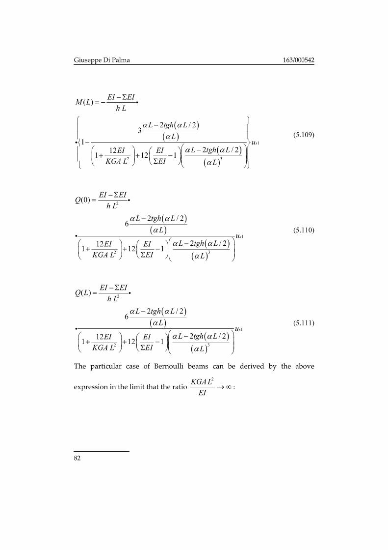
The particular case of Bernoulli beams can be derived by the above
expression in the limit that the ratio 2KGAL
EI→∞ :
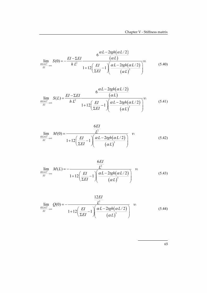
Page 72
Chapter V ‐ Stiffness matrix
65
( )( )
( )( )
212
3
2 / 26
lim (0)2 / 2
1 12 1KGALEI
L tgh LLEI EIS v
h L L tgh LEIEI L
α αα
α αα
→∞
−
−Σ= −
⎛ ⎞−⎛ ⎞+ − ⎜ ⎟⎜ ⎟⎜ ⎟Σ⎝ ⎠⎝ ⎠
(5.40)
( )( )
( )( )
212
3
2 / 26
lim ( )2 / 2
1 12 1KGALEI
L tgh LLEI EIS L v
h L L tgh LEIEI L
α αα
α αα
→∞
−
−Σ=
⎛ ⎞−⎛ ⎞+ − ⎜ ⎟⎜ ⎟⎜ ⎟Σ⎝ ⎠⎝ ⎠
(5.41)
( )( )
2
21
3
6
lim (0)2 / 2
1 12 1KGALEI
EILM vL tgh LEI
EI Lα α
α→∞
=⎛ ⎞−⎛ ⎞+ − ⎜ ⎟⎜ ⎟⎜ ⎟Σ⎝ ⎠⎝ ⎠
(5.42)
( )( )
2
21
3
6
lim ( )2 / 2
1 12 1KGALEI
EILM L vL tgh LEI
EI Lα α
α→∞
= −⎛ ⎞−⎛ ⎞+ − ⎜ ⎟⎜ ⎟⎜ ⎟Σ⎝ ⎠⎝ ⎠
(5.43)
( )( )
2
31
3
12
lim (0)2 / 2
1 12 1KGALEI
EILQ vL tgh LEI
EI Lα α
α→∞
= −⎛ ⎞−⎛ ⎞+ − ⎜ ⎟⎜ ⎟⎜ ⎟Σ⎝ ⎠⎝ ⎠
(5.44)
Page 73
Giuseppe Di Palma 163/000542
66
( )( )
2
31
3
12
lim ( )2 / 2
1 12 1KGALEI
EILQ L vL tgh LEI
EI Lα α
α→∞
= −⎛ ⎞−⎛ ⎞+ − ⎜ ⎟⎜ ⎟⎜ ⎟Σ⎝ ⎠⎝ ⎠
(5.45)
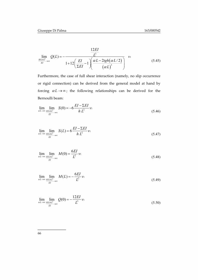
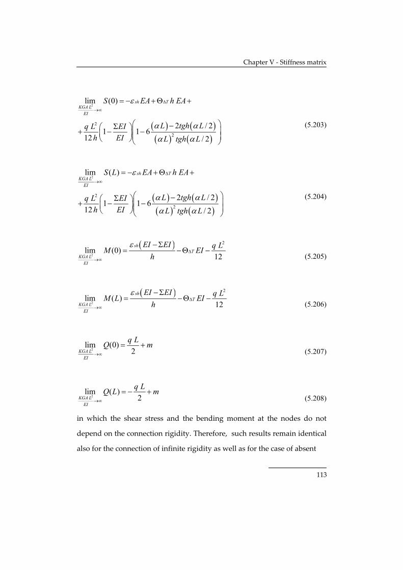
Furthermore, the case of full shear interaction (namely, no slip occurrence
or rigid connection) can be derived from the general model at hand by
forcing Lα →∞ ; the following relationships can be derived for the
Bernoulli beam:
212lim lim (0) 6
L KGALEI
EI EIS vh Lα →∞
→∞
−Σ= −
(5.46)
212lim lim ( ) 6
L KGALEI
EI EIS L vh Lα →∞
→∞
−Σ=
(5.47)
212
6lim lim (0)L KGAL
EI
EIM vLα →∞
→∞
= (5.48)
212
6lim lim ( )L KGAL
EI
EIM L vLα →∞
→∞
= − (5.49)
213
12lim lim (0)L KGAL
EI
EIQ vLα →∞
→∞
= − (5.50)
Page 74
Chapter V ‐ Stiffness matrix
67
213
12lim lim ( )L KGAL
EI
EIQ L vLα →∞
→∞
= − (5.51)
On the contrary, the general model reproduces the case of absent
interaction as 0Lα → :
20lim lim (0) 0L KGAL
EI
Sα →
→∞
= (5.52)
20lim lim ( ) 0L KGAL
EI
S Lα →
→∞
= (5.53)
2120
6lim lim (0)L KGAL
EI
EIM vLα →
→∞
Σ=
(5.54)
2120
6lim lim ( )L KGAL
EI
EIM L vLα →
→∞
Σ= −
(5.55)
2130
12lim lim (0)L KGAL
EI
EIQ vLα →
→∞
Σ= −
(5.56)
2130
12lim lim ( )L KGAL
EI
EIQ L vLα →
→∞
Σ= −
(5.57)
Finally, coming back to the general definition of stiffness terms in equation
(5.5), the terms of the first column of the stiffness matrix are listed below:
Page 75
Giuseppe Di Palma 163/000542
68
( )( )
11 3
32
12 12 / 2121 12 1
EIKL L tgh LEI EI
KGA L EI Lα α
α
=⎛ ⎞−⎛ ⎞ ⎛ ⎞+ + − ⎜ ⎟⎜ ⎟⎜ ⎟ ⎜ ⎟Σ⎝ ⎠⎝ ⎠ ⎝ ⎠
(5.58)
( )( )
21 2
32
6 12 / 2121 12 1
EIKL L tgh LEI EI
KGA L EI Lα α
α
= −⎛ ⎞−⎛ ⎞ ⎛ ⎞+ + − ⎜ ⎟⎜ ⎟⎜ ⎟ ⎜ ⎟Σ⎝ ⎠⎝ ⎠ ⎝ ⎠
(5.59)
( )( )
( )( )
31 2
32
2 / 26
2 / 2121 12 1
EI EIKh L
L tgh LL
L tgh LEI EIKGA L EI L
α αα
α αα
−Σ= −
−
⎛ ⎞−⎛ ⎞ ⎛ ⎞+ + − ⎜ ⎟⎜ ⎟⎜ ⎟ ⎜ ⎟Σ⎝ ⎠⎝ ⎠ ⎝ ⎠
i
i (5.60)
( )( )
41 3
32
12 12 / 2121 12 1
EIKL L tgh LEI EI
KGA L EI Lα α
α
= −⎛ ⎞−⎛ ⎞ ⎛ ⎞+ + − ⎜ ⎟⎜ ⎟⎜ ⎟ ⎜ ⎟Σ⎝ ⎠⎝ ⎠ ⎝ ⎠
(5.61)
( )( )
51 2
32
6 12 / 2121 12 1
EIKL L tgh LEI EI
KGA L EI Lα α
α
= −⎛ ⎞−⎛ ⎞ ⎛ ⎞+ + − ⎜ ⎟⎜ ⎟⎜ ⎟ ⎜ ⎟Σ⎝ ⎠⎝ ⎠ ⎝ ⎠
(5.62)
Page 76
Chapter V ‐ Stiffness matrix
69
( )( )
( )( )
61 2
32
2 / 26
2 / 2121 12 1
EI EIKh L
L tgh LL
L tgh LEI EIKGA L EI L
α αα
α αα
−Σ= −
−
⎛ ⎞−⎛ ⎞ ⎛ ⎞+ + − ⎜ ⎟⎜ ⎟⎜ ⎟ ⎜ ⎟Σ⎝ ⎠⎝ ⎠ ⎝ ⎠
i
i (5.63)
5.2.3 Stiffness matrix: the second column
Considering a nodal displacement vector D=[0,φ1,0,0,0,0] in equation
(5.14) the terms of the second column can be determined by equations
(5.22)÷(5.27).The constant Ci can be derived by solving those equations to
obtain the following results:
( )( )
( )
2
1 1
32
6 1
2 / 2121 12 1
EIEIL
CL tgh LEI EI
KGA L EI L
α αϕ
α αα
⎛ ⎞−⎜ ⎟Σ⎝ ⎠= −
⎛ ⎞−⎛ ⎞ ⎛ ⎞+ + − ⎜ ⎟⎜ ⎟⎜ ⎟ ⎜ ⎟Σ⎝ ⎠⎝ ⎠ ⎝ ⎠
(5.64)
( )( )
( )( )
2
2 1
32
/ 26 1
2 / 2121 12 1
tgh LEIEI L
CL tgh LEI EI
KGA L EI L
αα α
ϕα α
α
⎛ ⎞−⎜ ⎟Σ⎝ ⎠=
⎛ ⎞−⎛ ⎞ ⎛ ⎞+ + − ⎜ ⎟⎜ ⎟⎜ ⎟ ⎜ ⎟Σ⎝ ⎠⎝ ⎠ ⎝ ⎠
(5.65)
Page 77
Giuseppe Di Palma 163/000542
70
( )( )
23 1
32
1
2 / 2121 12 1
LCL tgh LEI EI
KGA L EI L
ϕα α
α
= −⎛ ⎞−⎛ ⎞ ⎛ ⎞+ + − ⎜ ⎟⎜ ⎟⎜ ⎟ ⎜ ⎟Σ⎝ ⎠⎝ ⎠ ⎝ ⎠
(5.66)
( )( )
4
1
32
12
312 / 2121 12 1
CL
L tgh LEI EIKGA L EI L
ϕα α
α
=
⎧ ⎫⎪ ⎪⎪ ⎪+⎨ ⎬
⎛ ⎞−⎛ ⎞⎪ ⎪⎛ ⎞+ + − ⎜ ⎟⎜ ⎟⎜ ⎟⎪ ⎪⎜ ⎟Σ⎝ ⎠⎝ ⎠ ⎝ ⎠⎩ ⎭
i
i (5.67)
{
( )( )
( )
5
22
1
32
1
6 6 1
2 / 2121 12 1
C
EI EIKGA L EIL
L tgh LEI EIKGA L EI L
αϕ
α αα
= − +
⎫⎡ ⎤⎛ ⎞ ⎪+ −⎢ ⎥⎜ ⎟Σ⎝ ⎠ ⎪⎢ ⎥⎣ ⎦+ ⎬⎛ ⎞−⎛ ⎞ ⎪⎛ ⎞+ + − ⎜ ⎟⎜ ⎟⎜ ⎟ ⎪⎜ ⎟Σ⎝ ⎠⎝ ⎠ ⎝ ⎠⎭
(5.68)
( )( )
( )( )
2
6 1
32
/ 26 1
2 / 2121 12 1
tgh LEIEI L
CL tgh LEI EI
KGA L EI L
αα α
ϕα α
α
⎛ ⎞−⎜ ⎟Σ⎝ ⎠= −
⎛ ⎞−⎛ ⎞ ⎛ ⎞+ + − ⎜ ⎟⎜ ⎟⎜ ⎟ ⎜ ⎟Σ⎝ ⎠⎝ ⎠ ⎝ ⎠
(5.69)
The consequent nodal stresses result as:
Page 78
Chapter V ‐ Stiffness matrix
71
( )( )
( )( )
1
32
(0)
2 / 23
12 / 2121 12 1
EI EISh L
L tgh LL
L tgh LEI EIKGA L EI L
α αα
ϕα α
α
−Σ=
⎧ ⎫−⎪ ⎪⎪ ⎪+⎨ ⎬
⎛ ⎞−⎛ ⎞⎪ ⎪⎛ ⎞+ + − ⎜ ⎟⎜ ⎟⎜ ⎟⎪ ⎪⎜ ⎟Σ⎝ ⎠⎝ ⎠ ⎝ ⎠⎩ ⎭
i
i (5.70)
( )( )
( )( )
1
32
( )
2 / 23
12 / 2121 12 1
EI EIS Lh L
L tgh LL
L tgh LEI EIKGA L EI L
α αα
ϕα α
α
−Σ=
⎧ ⎫−⎪ ⎪⎪ ⎪−⎨ ⎬
⎛ ⎞−⎛ ⎞⎪ ⎪⎛ ⎞+ + − ⎜ ⎟⎜ ⎟⎜ ⎟⎪ ⎪⎜ ⎟Σ⎝ ⎠⎝ ⎠ ⎝ ⎠⎩ ⎭
i
i (5.71)
( )( )
1
32
(0)
312 / 2121 12 1
EIML
L tgh LEI EIKGA L EI L
ϕα α
α
= −
⎧ ⎫⎪ ⎪⎪ ⎪+⎨ ⎬
⎛ ⎞−⎛ ⎞⎪ ⎪⎛ ⎞+ + − ⎜ ⎟⎜ ⎟⎜ ⎟⎪ ⎪⎜ ⎟Σ⎝ ⎠⎝ ⎠ ⎝ ⎠⎩ ⎭
i
i (5.72)
Page 79
Giuseppe Di Palma 163/000542
72
( )( )
1
32
( )
312 / 2121 12 1
EIM LL
L tgh LEI EIKGA L EI L
ϕα α
α
= −
⎧ ⎫⎪ ⎪⎪ ⎪−⎨ ⎬
⎛ ⎞−⎛ ⎞⎪ ⎪⎛ ⎞+ + − ⎜ ⎟⎜ ⎟⎜ ⎟⎪ ⎪⎜ ⎟Σ⎝ ⎠⎝ ⎠ ⎝ ⎠⎩ ⎭
i
i (5.73)
( )( )
2
1
32
6(0)
12 / 2121 12 1
EIQL
L tgh LEI EIKGA L EI L
ϕα α
α
=
⎛ ⎞−⎛ ⎞ ⎛ ⎞+ + − ⎜ ⎟⎜ ⎟⎜ ⎟ ⎜ ⎟Σ⎝ ⎠⎝ ⎠ ⎝ ⎠
i
i (5.74)
( )( )
2
1
32
6( )
12 / 2121 12 1
EIQ LL
L tgh LEI EIKGA L EI L
ϕα α
α
=
⎛ ⎞−⎛ ⎞ ⎛ ⎞+ + − ⎜ ⎟⎜ ⎟⎜ ⎟ ⎜ ⎟Σ⎝ ⎠⎝ ⎠ ⎝ ⎠
i
i (5.75)
The particular case of Bernoulli beams can be derived by the above
expression in the limit that the ratio 2KGAL
EI→∞ :
Page 80
Chapter V ‐ Stiffness matrix
73
( )( )
( )( )
2
1
3
lim (0)
2 / 23
12 / 2
1 12 1
KGALEI
EI EISh L
L tgh LL
L tgh LEIEI L
α αα
ϕα α
α
→∞
−Σ=
⎧ ⎫−⎪ ⎪⎪ ⎪+⎨ ⎬
⎛ ⎞−⎪ ⎪⎛ ⎞+ − ⎜ ⎟⎜ ⎟⎪ ⎪⎜ ⎟Σ⎝ ⎠⎝ ⎠⎩ ⎭
i
i (5.76)
( )( )
( )( )
2
1
3
lim ( )
2 / 23
12 / 2
1 12 1
KGALEI
EI EIS Lh L
L tgh LL
L tgh LEIEI L
α αα
ϕα α
α
→∞
−Σ=
⎧ ⎫−⎪ ⎪⎪ ⎪−⎨ ⎬
⎛ ⎞−⎪ ⎪⎛ ⎞+ − ⎜ ⎟⎜ ⎟⎪ ⎪⎜ ⎟Σ⎝ ⎠⎝ ⎠⎩ ⎭
i
i (5.77)
( )( )
21
3
3lim (0) 12 / 2
1 12 1KGALEI
EIML L tgh LEI
EI L
ϕα α
α→∞
⎧ ⎫⎪ ⎪⎪ ⎪
= − +⎨ ⎬⎛ ⎞−⎪ ⎪⎛ ⎞+ − ⎜ ⎟⎜ ⎟⎪ ⎪⎜ ⎟Σ⎝ ⎠⎝ ⎠⎩ ⎭
(5.78)
Page 81
Giuseppe Di Palma 163/000542
74
( )( )
21
3
3lim ( ) 12 / 2
1 12 1KGALEI
EIM LL L tgh LEI
EI L
ϕα α
α→∞
⎧ ⎫⎪ ⎪⎪ ⎪
= − −⎨ ⎬⎛ ⎞−⎪ ⎪⎛ ⎞+ − ⎜ ⎟⎜ ⎟⎪ ⎪⎜ ⎟Σ⎝ ⎠⎝ ⎠⎩ ⎭
(5.79)
( )( )
212
3
6 1lim (0)2 / 2
1 12 1KGALEI
EIQL L tgh LEI
EI L
ϕα α
α→∞
=⎛ ⎞−⎛ ⎞+ − ⎜ ⎟⎜ ⎟⎜ ⎟Σ⎝ ⎠⎝ ⎠
(5.80)
( )( )
212
3
6 1lim ( )2 / 2
1 12 1KGALEI
EIQ LL L tgh LEI
EI L
ϕα α
α→∞
=⎛ ⎞−⎛ ⎞+ − ⎜ ⎟⎜ ⎟⎜ ⎟Σ⎝ ⎠⎝ ⎠
(5.81)
Furthermore, the case of full shear interaction (namely, no slip occurrence
or rigid connection) can be derived from the general model at hand by
forcing Lα →∞ ; the following relationships can be derived for the
Bernoulli beam:
21lim lim (0) 4
L KGALEI
EI EISh Lα
ϕ→∞
→∞
−Σ=
(5.82)
21lim lim ( ) 2
L KGALEI
EI EIS Lh Lα
ϕ→∞
→∞
−Σ= −
(5.83)
Page 82
Chapter V ‐ Stiffness matrix
75
21
4lim lim (0)L KGAL
EI
EIMLα
ϕ→∞
→∞
= − (5.84)
21
2lim lim ( )L KGAL
EI
EIM LLα
ϕ→∞
→∞
= (5.85)
212
6lim lim (0)L KGAL
EI
EIQLα
ϕ→∞
→∞
= (5.86)
212
6lim lim ( )L KGAL
EI
EIQ LLα
ϕ→∞
→∞
= (5.87)
On the contrary, the general model reproduces the case of absent
interaction as 0Lα → :
21lim lim (0)
L KGALEI
EI EISh Lα
ϕ→∞
→∞
−Σ=
(5.88)
21lim lim ( )
L KGALEI
EI EIS Lh Lα
ϕ→∞
→∞
−Σ=
(5.89)
21
3lim lim (0)L KGAL
EI
EI EIMLα
ϕ→∞
→∞
+ Σ⎛ ⎞= −⎜ ⎟⎝ ⎠
(5.90)
Page 83
Giuseppe Di Palma 163/000542
76
21
3lim lim ( )L KGAL
EI
EI EIM LLα
ϕ→∞
→∞
− Σ⎛ ⎞= −⎜ ⎟⎝ ⎠
(5.91)
212
6lim lim (0)L KGAL
EI
EIQLα
ϕ→∞
→∞
Σ=
(5.92)
212
6lim lim ( )L KGAL
EI
EIQ LLα
ϕ→∞
→∞
Σ=
(5.93)
Finally, coming back to the general definition of stiffness terms in equation
(5.5), the terms of the first column of the stiffness matrix are listed below:
( )( )
12 2
32
6 12 / 2121 12 1
EIKL L tgh LEI EI
KGA L EI Lα α
α
= −⎛ ⎞−⎛ ⎞ ⎛ ⎞+ + − ⎜ ⎟⎜ ⎟⎜ ⎟ ⎜ ⎟Σ⎝ ⎠⎝ ⎠ ⎝ ⎠
(5.94)
( )( )
22
32
312 / 2121 12 1
EIKL
L tgh LEI EIKGA L EI L
α αα
=
⎧ ⎫⎪ ⎪⎪ ⎪+⎨ ⎬
⎛ ⎞−⎛ ⎞⎪ ⎪⎛ ⎞+ + − ⎜ ⎟⎜ ⎟⎜ ⎟⎪ ⎪⎜ ⎟Σ⎝ ⎠⎝ ⎠ ⎝ ⎠⎩ ⎭
i
i (5.95)
Page 84
Chapter V ‐ Stiffness matrix
77
( )( )
( )( )
32
32
2 / 23
12 / 2121 12 1
EI EIKh L
L tgh LL
L tgh LEI EIKGA L EI L
α αα
α αα
−Σ=
⎧ ⎫−⎪ ⎪⎪ ⎪+⎨ ⎬
⎛ ⎞−⎛ ⎞⎪ ⎪⎛ ⎞+ + − ⎜ ⎟⎜ ⎟⎜ ⎟⎪ ⎪⎜ ⎟Σ⎝ ⎠⎝ ⎠ ⎝ ⎠⎩ ⎭
i
i (5.96)
( )( )
42 2
32
6 12 / 2121 12 1
EIKL L tgh LEI EI
KGA L EI Lα α
α
=⎛ ⎞−⎛ ⎞ ⎛ ⎞+ + − ⎜ ⎟⎜ ⎟⎜ ⎟ ⎜ ⎟Σ⎝ ⎠⎝ ⎠ ⎝ ⎠
(5.97)
( )( )
52
32
312 / 2121 12 1
EIKL
L tgh LEI EIKGA L EI L
α αα
=
⎧ ⎫⎪ ⎪⎪ ⎪− +⎨ ⎬
⎛ ⎞−⎛ ⎞⎪ ⎪⎛ ⎞+ + − ⎜ ⎟⎜ ⎟⎜ ⎟⎪ ⎪⎜ ⎟Σ⎝ ⎠⎝ ⎠ ⎝ ⎠⎩ ⎭
i
i (5.98)
( )( )
( )( )
62
32
2 / 23
12 / 2121 12 1
EI EIKh L
L tgh LL
L tgh LEI EIKGA L EI L
α αα
α αα
−Σ=
⎧ ⎫−⎪ ⎪⎪ ⎪− +⎨ ⎬
⎛ ⎞−⎛ ⎞⎪ ⎪⎛ ⎞+ + − ⎜ ⎟⎜ ⎟⎜ ⎟⎪ ⎪⎜ ⎟Σ⎝ ⎠⎝ ⎠ ⎝ ⎠⎩ ⎭
i
i (5.99)
Page 85
Giuseppe Di Palma 163/000542
78
5.2.4 Stiffness matrix: the third column
Considering a nodal displacement vector D=[0,0,us1,0,0,0] in equation
(5.14) the terms of the second column can be determined by equations
(5.22)÷(5.27). The constant Ci can be derived by solving those equations to
obtain the following results:
( )( )
( )( )
1 3
3
1
32
2 / 26 1
12 / 2121 12 1
s
s
k hCEI
L tgh LEIEI L
uL tgh LEI EI
KGA L EI L
α
α αα
α αα
=Σ
⎧ ⎫⎛ ⎞−⎛ ⎞⎪ ⎪− ⎜ ⎟⎜ ⎟⎜ ⎟Σ⎝ ⎠⎪ ⎪⎝ ⎠−⎨ ⎬⎛ ⎞−⎛ ⎞⎪ ⎪⎛ ⎞+ + − ⎜ ⎟⎜ ⎟⎜ ⎟⎪ ⎪⎜ ⎟Σ⎝ ⎠⎝ ⎠ ⎝ ⎠⎩ ⎭
i
i (5.100)
( ){
( )( )
( )
( )( )
2 3
3
1
32
2 / 26 1 / 2
2 / 2121 12 1
s
ks hC ctgh LEI
L tgh LEI tgh LEI L
uL tgh LEI EI
KGA L EI L
αα
α αα
α
α αα
= − +Σ
⎫⎛ ⎞−⎛ ⎞ ⎪− ⎜ ⎟⎜ ⎟⎜ ⎟Σ⎝ ⎠ ⎪⎝ ⎠+ ⎬⎛ ⎞−⎛ ⎞ ⎪⎛ ⎞+ + − ⎜ ⎟⎜ ⎟⎜ ⎟ ⎪⎜ ⎟Σ⎝ ⎠⎝ ⎠ ⎝ ⎠⎭
(5.101)
( )( )
( )( )
3
3 1
32
2 / 2
2 / 2121 12 1
s
L tgh Lks hEI L
C uL tgh LEI EI
KGA L EI L
α αα
α αα
⎛ ⎞−⎛ ⎞⎜ ⎟⎜ ⎟⎜ ⎟Σ⎝ ⎠⎝ ⎠= −
⎛ ⎞−⎛ ⎞ ⎛ ⎞+ + − ⎜ ⎟⎜ ⎟⎜ ⎟ ⎜ ⎟Σ⎝ ⎠⎝ ⎠ ⎝ ⎠
(5.102)
Page 86
Chapter V ‐ Stiffness matrix
79
( ) ( )
( )( )
( )( )
4
1
- 22
- 2 / 2 1818 -1 3 2
- 2 / 2121 12 -12 3
s
tgh aL aL tgh aLks hCaL aLEI a L
aL tgh aLEI EISEI KGA LaL
uaL tgh aLEI EI
SEIKGA L aL
⎧ ⎛ ⎞= +⎨ ⎜ ⎟
⎩ ⎝ ⎠Σ
⎫⎛ ⎞⎛ ⎞ ⎪⎜ ⎟ +⎜ ⎟ ⎪⎜ ⎟⎝ ⎠ ⎪⎝ ⎠⎬
⎛ ⎞⎛ ⎞ ⎪⎛ ⎞⎜ ⎟⎜ ⎟+ + ⎪⎜ ⎟⎜ ⎟ ⎜ ⎟⎝ ⎠ ⎪⎝ ⎠ ⎝ ⎠⎭
i
i
(5.103)
( )( )
( )( )
( )
5 2
2 2
1
32
2 / 26 61
12 / 2121 12 1
s
s
k hCEI
L tgh LEI EIEI KGA L LL
uL tgh LEI EI
KGA L EI L
α
α ααα
α αα
=Σ
⎧ ⎫⎛ ⎞⎛ ⎞−⎛ ⎞⎪ ⎪− +⎜ ⎟⎜ ⎟⎜ ⎟⎜ ⎟Σ⎝ ⎠⎪ ⎪⎝ ⎠⎝ ⎠− +⎨ ⎬⎛ ⎞−⎛ ⎞⎪ ⎪⎛ ⎞+ + − ⎜ ⎟⎜ ⎟⎜ ⎟⎪ ⎪⎜ ⎟Σ⎝ ⎠⎝ ⎠ ⎝ ⎠⎩ ⎭
i
i
(5.104)
( ){
( )( )
( )
( )( )
6 3
3
1
32
2 / 26 1 / 2
2 / 2121 12 1
s
s
k hC ctgh LEI
L tgh LEI tgh LEI L
uL tgh LEI EI
KGA L EI L
αα
α αα
α
α αα
= +Σ
⎫⎛ ⎞−⎛ ⎞ ⎪− ⎜ ⎟⎜ ⎟⎜ ⎟Σ⎝ ⎠ ⎪⎝ ⎠− ⎬⎛ ⎞−⎛ ⎞ ⎪⎛ ⎞+ + − ⎜ ⎟⎜ ⎟⎜ ⎟ ⎪⎜ ⎟Σ⎝ ⎠⎝ ⎠ ⎝ ⎠⎭
(5.105)
The consequent nodal stresses result as:
Page 87
Giuseppe Di Palma 163/000542
80
( )( )
( )( )
( )
( )( )
12
2 2
3
32
2
(0)
2 / 212 1
2 / 2121 12 1
12 1
sEI EIS uh L
L tgh LL EI EItgh L EI EIL
L tgh LEI EI EIKGA L EI EIL
L senh LEI EIEI EI L
α ααα α
α αα
α αα
•−Σ
=
⎧ ⎛ ⎞−Σ Σ⎛ ⎞ ⎛ ⎞⎪ + −⎜ ⎟⎜ ⎟ ⎜ ⎟⎜ ⎟⎪ ⎝ ⎠ ⎝ ⎠⎪ ⎝ ⎠ +⎨⎡ ⎤⎛ ⎞−⎛ ⎞⎪ Σ⎛ ⎞ ⎛ ⎞⎢ ⎥+ + − ⎜ ⎟⎜ ⎟ ⎜ ⎟⎜ ⎟⎪ ⎜ ⎟Σ⎝ ⎠ ⎝ ⎠⎢ ⎥⎝ ⎠ ⎝ ⎠⎪⎣ ⎦⎩
−Σ Σ⎛ ⎞⎛ ⎞−⎜ ⎟⎜ ⎟⎝ ⎠⎝ ⎠
+
i
( )( )
( )
( )
32
2
2
13
2 / 2121 12 1
12 1
2 /121 12 1
senh L
L tgh LEI EI EIKGA L EI EIL
EI EI EI EI LEI KGA L EI EI tgh L
L tgh LEI EIKGA L EI
α
α αα
αα
α α
⎛ ⎞+⎜ ⎟⎜ ⎟
⎝ ⎠ +⎡ ⎤⎛ ⎞−⎛ ⎞ Σ⎛ ⎞ ⎛ ⎞⎢ ⎥+ + − ⎜ ⎟⎜ ⎟ ⎜ ⎟⎜ ⎟ ⎜ ⎟Σ⎝ ⎠ ⎝ ⎠⎢ ⎥⎝ ⎠ ⎝ ⎠⎣ ⎦
⎡ ⎤⎛ ⎞Σ Σ Σ⎛ ⎞ ⎛ ⎞ ⎛ ⎞− +⎢ ⎥⎜ ⎟ ⎜ ⎟ ⎜ ⎟⎜ ⎟⎝ ⎠ ⎝ ⎠ ⎝ ⎠⎝ ⎠ ⎣ ⎦+
−⎛ ⎞ ⎛ ⎞+ + −⎜ ⎟⎜ ⎟ Σ⎝ ⎠⎝ ⎠
( )( )3
2 EIEILα
⎫⎪⎪⎪⎬
⎡ ⎤⎛ ⎞ ⎪Σ⎛ ⎞⎢ ⎥⎜ ⎟ ⎜ ⎟⎪⎜ ⎟ ⎝ ⎠⎢ ⎥⎝ ⎠ ⎪⎣ ⎦ ⎭
(5.106)
Page 88
Chapter V ‐ Stiffness matrix
81
( )( )
( )( )
( )
( )
12
2 2
3
32
( )
2 / 212 1
2 / 2121 12 1
cos12 1
sEI EIS L uh L
L tgh LL EI EIsenh L EI EIL
L tgh LEI EI EIKGA L EI EIL
L L senEI EIEI EI
α ααα α
α αα
α α
•−Σ
=
⎧ ⎛ ⎞−Σ Σ⎛ ⎞ ⎛ ⎞⎪ + −⎜ ⎟⎜ ⎟ ⎜ ⎟⎜ ⎟⎪ ⎝ ⎠ ⎝ ⎠⎪ ⎝ ⎠ +⎨⎡ ⎤⎛ ⎞−⎛ ⎞⎪ Σ⎛ ⎞ ⎛ ⎞⎢ ⎥+ + − ⎜ ⎟⎜ ⎟ ⎜ ⎟⎜ ⎟⎪ ⎜ ⎟Σ⎝ ⎠ ⎝ ⎠⎢ ⎥⎝ ⎠ ⎝ ⎠⎪ ⎣ ⎦⎩
−Σ Σ⎛ ⎞⎛ ⎞−⎜ ⎟⎜ ⎟⎝ ⎠⎝ ⎠
+
i
( )( ) ( )
( )( )
( )
2
32
2
2
16
2 / 2121 12 1
12 1
121 12 1
h LL senh L
L tgh LEI EI EIKGA L EI EIL
EI EI EI EI LEI KGA L EI EI senh L
LEI EIKGA L EI
αα α
α αα
αα
α
⎛ ⎞−⎜ ⎟⎜ ⎟
⎝ ⎠ +⎡ ⎤⎛ ⎞−⎛ ⎞ Σ⎛ ⎞ ⎛ ⎞⎢ ⎥+ + − ⎜ ⎟⎜ ⎟ ⎜ ⎟⎜ ⎟ ⎜ ⎟Σ⎝ ⎠ ⎝ ⎠⎢ ⎥⎝ ⎠ ⎝ ⎠⎣ ⎦
⎡ ⎤⎛ ⎞Σ Σ Σ⎛ ⎞ ⎛ ⎞ ⎛ ⎞− +⎢ ⎥⎜ ⎟ ⎜ ⎟ ⎜ ⎟⎜ ⎟⎝ ⎠ ⎝ ⎠ ⎝ ⎠⎝ ⎠ ⎣ ⎦+
−⎛ ⎞ ⎛ ⎞+ + −⎜ ⎟⎜ ⎟ Σ⎝ ⎠⎝ ⎠
( )( )3
2 / 2tgh L EIEIL
αα
⎫⎪⎪⎪⎬
⎡ ⎤⎛ ⎞ ⎪Σ⎛ ⎞⎢ ⎥⎜ ⎟ ⎜ ⎟⎪⎜ ⎟ ⎝ ⎠⎢ ⎥⎝ ⎠ ⎪⎣ ⎦ ⎭
(5.107)
( )( )
( )( )
1
32
(0)
2 / 23
12 / 2121 12 1
s
EI EIMh L
L tgh LL
uL tgh LEI EI
KGA L EI L
α αα
α αα
−Σ= −
⎧ ⎫−⎪ ⎪⎪ ⎪+⎨ ⎬
⎛ ⎞−⎛ ⎞⎪ ⎪⎛ ⎞+ + − ⎜ ⎟⎜ ⎟⎜ ⎟⎪ ⎪⎜ ⎟Σ⎝ ⎠⎝ ⎠ ⎝ ⎠⎩ ⎭
i
i (5.108)
Page 89
Giuseppe Di Palma 163/000542
82
( )( )
( )( )
1
32
( )
2 / 23
12 / 2121 12 1
s
EI EIM Lh L
L tgh LL
uL tgh LEI EI
KGA L EI L
α αα
α αα
−Σ= −
⎧ ⎫−⎪ ⎪⎪ ⎪−⎨ ⎬
⎛ ⎞−⎛ ⎞⎪ ⎪⎛ ⎞+ + − ⎜ ⎟⎜ ⎟⎜ ⎟⎪ ⎪⎜ ⎟Σ⎝ ⎠⎝ ⎠ ⎝ ⎠⎩ ⎭
i
i (5.109)
( )( )
( )( )
2
1
32
(0)
2 / 26
2 / 2121 12 1
s
EI EIQh L
L tgh LL
uL tgh LEI EI
KGA L EI L
α αα
α αα
−Σ=
−
⎛ ⎞−⎛ ⎞ ⎛ ⎞+ + − ⎜ ⎟⎜ ⎟⎜ ⎟ ⎜ ⎟Σ⎝ ⎠⎝ ⎠ ⎝ ⎠
i
i (5.110)
( )( )
( )( )
2
1
32
( )
2 / 26
2 / 2121 12 1
s
EI EIQ Lh L
L tgh LL
uL tgh LEI EI
KGA L EI L
α αα
α αα
−Σ=
−
⎛ ⎞−⎛ ⎞ ⎛ ⎞+ + − ⎜ ⎟⎜ ⎟⎜ ⎟ ⎜ ⎟Σ⎝ ⎠⎝ ⎠ ⎝ ⎠
i
i (5.111)
The particular case of Bernoulli beams can be derived by the above
expression in the limit that the ratio 2KGAL
EI→∞ :
Page 90
Chapter V ‐ Stiffness matrix
83
( )( )
( )( )
( )
( )( ) ( )
2 2
2 2
3
3
2
lim (0)
2 / 212 1
2 / 21 12 1
12 1
KGALEI
EI EISh L
L tgh LL EI EItgh L EI EIL
L tgh LEI EIEI EIL
L senh LEI EIEI EI L senh L
α ααα α
α αα
α αα α
→∞
−Σ=
⎧ ⎛ ⎞−Σ Σ⎛ ⎞ ⎛ ⎞⎪ + −⎜ ⎟⎜ ⎟ ⎜ ⎟⎜ ⎟⎪ ⎝ ⎠ ⎝ ⎠⎪ ⎝ ⎠ +⎨⎡ ⎤⎛ ⎞−⎪ Σ⎛ ⎞ ⎛ ⎞⎢ ⎥+ − ⎜ ⎟⎜ ⎟ ⎜ ⎟⎪ ⎜ ⎟Σ⎝ ⎠ ⎝ ⎠⎢ ⎥⎝ ⎠⎪ ⎣ ⎦⎩
−Σ Σ⎛ ⎞⎛ ⎞− +⎜ ⎟⎜ ⎟⎝ ⎠⎝ ⎠
+
i
i
( )( )
1
3
13
2 / 21 12 1
suL tgh LEI EI
EI EILα α
α
⎫⎛ ⎞⎪⎜ ⎟⎜ ⎟ ⎪⎪⎝ ⎠⎬
⎡ ⎤⎛ ⎞− ⎪Σ⎛ ⎞ ⎛ ⎞⎢ ⎥+ − ⎜ ⎟⎜ ⎟ ⎜ ⎟⎪⎜ ⎟Σ⎝ ⎠ ⎝ ⎠⎢ ⎥⎝ ⎠ ⎪⎣ ⎦ ⎭
(5.112)
( )( )
( )( )
( )
( ) ( )( )
2 2
2 2
3
3
2
lim ( )
2 / 212 1
2 / 21 12 1
cos12 1
KGALEI
EI EIS Lh L
L tgh LL EI EIsenh L EI EIL
L tgh LEI EIEI EIL
L L senh LEI EIEI EI L s
α ααα α
α αα
α α αα
→∞
−Σ=
⎧ ⎛ ⎞−Σ Σ⎛ ⎞ ⎛ ⎞⎪ + −⎜ ⎟⎜ ⎟ ⎜ ⎟⎜ ⎟⎪ ⎝ ⎠ ⎝ ⎠⎪ ⎝ ⎠ +⎨⎡ ⎤⎛ ⎞−⎪ Σ⎛ ⎞ ⎛ ⎞⎢ ⎥+ − ⎜ ⎟⎜ ⎟ ⎜ ⎟⎪ ⎜ ⎟Σ⎝ ⎠ ⎝ ⎠⎢ ⎥⎝ ⎠⎪ ⎣ ⎦⎩
−Σ Σ⎛ ⎞⎛ ⎞−⎜ ⎟⎜ ⎟⎝ ⎠⎝ ⎠
+
i
i
( )( )
( )
1
3
16
2 / 21 12 1
senh L
uL tgh LEI EI
EI EIL
α
α αα
⎫⎛ ⎞⎪−⎜ ⎟⎜ ⎟⎪⎪⎝ ⎠⎬
⎡ ⎤⎛ ⎞− ⎪Σ⎛ ⎞ ⎛ ⎞⎢ ⎥+ − ⎜ ⎟⎜ ⎟ ⎜ ⎟ ⎪⎜ ⎟Σ⎝ ⎠ ⎝ ⎠⎢ ⎥⎝ ⎠ ⎪⎣ ⎦ ⎭
(5.113)
Page 91
Giuseppe Di Palma 163/000542
84
( )( )
( )( )
2
1
3
lim (0)
2 / 23
12 / 2
1 12 1
KGALEI
s
EI EIMh L
L tgh LL
uL tgh LEI
EI L
α αα
α αα
→∞
−Σ= −
⎧ ⎫−⎪ ⎪⎪ ⎪+⎨ ⎬
⎛ ⎞−⎪ ⎪⎛ ⎞+ − ⎜ ⎟⎜ ⎟⎪ ⎪⎜ ⎟Σ⎝ ⎠⎝ ⎠⎩ ⎭
i
i
(5.114)
( )( )
( )( )
2
1
3
lim ( )
2 / 23
12 / 2
1 12 1
KGALEI
s
EI EIM Lh L
L tgh LL
uL tgh LEI
EI L
α αα
α αα
→∞
−Σ= −
⎧ ⎫−⎪ ⎪⎪ ⎪−⎨ ⎬
⎛ ⎞−⎪ ⎪⎛ ⎞+ − ⎜ ⎟⎜ ⎟⎪ ⎪⎜ ⎟Σ⎝ ⎠⎝ ⎠⎩ ⎭
i
i
(5.115)
( )( )
( )( )
212
3
2 / 26
lim (0)2 / 2
1 12 1
sKGALEI
L tgh LLEI EIQ u
h L L tgh LEIEI L
α αα
α αα
→∞
−
−Σ=
⎛ ⎞−⎛ ⎞+ − ⎜ ⎟⎜ ⎟⎜ ⎟Σ⎝ ⎠⎝ ⎠
(5.116)
( )( )
( )( )
212
3
2 / 26
lim ( )2 / 2
1 12 1
sKGALEI
L tgh LLEI EIQ L u
h L L tgh LEIEI L
α αα
α αα
→∞
−
−Σ=
⎛ ⎞−⎛ ⎞+ − ⎜ ⎟⎜ ⎟⎜ ⎟Σ⎝ ⎠⎝ ⎠
(5.117)
Page 92
Chapter V ‐ Stiffness matrix
85
The above general expressions basically reduce to the ones derived by
Faella, Martinelli and Nigro (2002) within the framework of the Newmark
theory as 2KGAL
EI→∞ .
Furthermore, the case of full shear interaction (namely, no slip occurrence
or rigid connection) can be derived from the general model at hand by
forcing Lα →∞ ; the following relationships can be derived for the
Bernoulli beam:
2lim lim (0)L KGAL
EI
Sα →∞
→∞
= +∞ (5.118)
( )2
2
12lim lim ( ) 2 sL KGAL
EI
EI EIS L u
EI h Lα →∞→∞
−Σ= − (5.119)
( )2
1lim lim (0) 4 sL KGAL
EI
EI EIM u
h Lα →∞→∞
−Σ= −
(5.120)
( )2
1lim lim ( ) 2 sL KGAL
EI
EI EIM L u
h Lα →∞→∞
−Σ=
(5.121)
( )2
12lim lim (0) 6 sL KGAL
EI
EI EIQ u
h Lα →∞→∞
−Σ=
(5.122)
Page 93
Giuseppe Di Palma 163/000542
86
( )2
12lim lim ( ) 6 sL KGAL
EI
EI EIQ L u
h Lα →∞→∞
−Σ=
(5.123)
On the contrary, the general model reproduces the case of absent
interaction as 0Lα → :
2120
lim lim (0) sL KGAL
EI
EI EIS uh Lα →
→∞
−Σ=
(5.124)
2120
lim lim ( ) sL KGAL
EI
EI EIS L uh Lα →
→∞
−Σ=
(5.125)
21
0lim lim (0) sL KGAL
EI
EI EIM uh Lα →
→∞
−Σ= −
(5.126)
21
0lim lim ( ) sL KGAL
EI
EI EIM L uh Lα →
→∞
−Σ= −
(5.127)
20lim lim (0) 0L KGAL
EI
Qα →
→∞
= (5.128)
20lim lim ( ) 0L KGAL
EI
Q Lα →
→∞
= (5.129)
Finally, coming back to the general definition of stiffness terms in equation
(5.5), the terms of the first column of the stiffness matrix are listed below:
Page 94
Chapter V ‐ Stiffness matrix
87
( )( )
( )( )
13 2
32
2 / 26
2 / 2121 12 1
EI EIKh L
L tgh LL
L tgh LEI EIKGA L EI L
α αα
α αα
−Σ= −
−
⎛ ⎞−⎛ ⎞ ⎛ ⎞+ + − ⎜ ⎟⎜ ⎟⎜ ⎟ ⎜ ⎟Σ⎝ ⎠⎝ ⎠ ⎝ ⎠
i
i (5.130)
( )( )
( )( )
23
32
2 / 23
12 / 2121 12 1
EI EIKh L
L tgh LL
L tgh LEI EIKGA L EI L
α αα
α αα
−Σ=
⎧ ⎫−⎪ ⎪⎪ ⎪+⎨ ⎬
⎛ ⎞−⎛ ⎞⎪ ⎪⎛ ⎞+ + − ⎜ ⎟⎜ ⎟⎜ ⎟⎪ ⎪⎜ ⎟Σ⎝ ⎠⎝ ⎠ ⎝ ⎠⎩ ⎭
i
i (5.131)
Page 95
Giuseppe Di Palma 163/000542
88
( )( )
( )( )
( )
( )( )
33 2
2 2
3
32
2
2 / 212 1
2 / 2121 12 1
12 1
EI EIKh L
L tgh LL EI EItgh L EI EIL
L tgh LEI EI EIKGA L EI EIL
L senh LEI EIEI EI L senh
α ααα α
α αα
α αα
−Σ=
⎧ ⎛ ⎞−Σ Σ⎛ ⎞ ⎛ ⎞⎪ + −⎜ ⎟⎜ ⎟ ⎜ ⎟⎜ ⎟⎪ ⎝ ⎠ ⎝ ⎠⎪ ⎝ ⎠ +⎨⎡ ⎤⎛ ⎞−⎛ ⎞⎪ Σ⎛ ⎞ ⎛ ⎞⎢ ⎥+ + − ⎜ ⎟⎜ ⎟ ⎜ ⎟⎜ ⎟⎪ ⎜ ⎟Σ⎝ ⎠ ⎝ ⎠⎢ ⎥⎝ ⎠ ⎝ ⎠⎪⎣ ⎦⎩
−Σ Σ⎛ ⎞⎛ ⎞−⎜ ⎟⎜ ⎟⎝ ⎠⎝ ⎠
+
i
i
( )( )
( )
( )( )
( )
32
2
32
13
2 / 2121 12 1
12 1
2 / 2121 12 1
L
L tgh LEI EI EIKGA L EI EIL
EI EI EI EI LEI KGA L EI EI tgh L
L tgh LEI EIKGA L EI L
α
α αα
αα
α αα
⎛ ⎞+⎜ ⎟⎜ ⎟
⎝ ⎠ +⎡ ⎤⎛ ⎞−⎛ ⎞ Σ⎛ ⎞ ⎛ ⎞⎢ ⎥+ + − ⎜ ⎟⎜ ⎟ ⎜ ⎟⎜ ⎟ ⎜ ⎟Σ⎝ ⎠ ⎝ ⎠⎢ ⎥⎝ ⎠ ⎝ ⎠⎣ ⎦
⎡ ⎤⎛ ⎞Σ Σ Σ⎛ ⎞ ⎛ ⎞ ⎛ ⎞− +⎢ ⎥⎜ ⎟ ⎜ ⎟ ⎜ ⎟⎜ ⎟⎝ ⎠ ⎝ ⎠ ⎝ ⎠⎝ ⎠ ⎣ ⎦+
−⎛ ⎞ ⎛ ⎞+ + −⎜ ⎟⎜ ⎟ Σ⎝ ⎠⎝ ⎠
EIEI
⎫⎪⎪⎪⎬
⎡ ⎤⎛ ⎞ ⎪Σ⎛ ⎞⎢ ⎥⎜ ⎟ ⎜ ⎟⎪⎜ ⎟ ⎝ ⎠⎢ ⎥⎝ ⎠ ⎪⎣ ⎦ ⎭
(5.132)
( )( )
( )( )
43 2
32
2 / 26
2 / 2121 12 1
EI EIKh L
L tgh LL
L tgh LEI EIKGA L EI L
α αα
α αα
−Σ=
−
⎛ ⎞−⎛ ⎞ ⎛ ⎞+ + − ⎜ ⎟⎜ ⎟⎜ ⎟ ⎜ ⎟Σ⎝ ⎠⎝ ⎠ ⎝ ⎠
i
i (5.133)
Page 96
Chapter V ‐ Stiffness matrix
89
( )( )
( )( )
53
32
2 / 23
12 / 2121 12 1
EI EIKh L
L tgh LL
L tgh LEI EIKGA L EI L
α αα
α αα
−Σ= −
⎧ ⎫−⎪ ⎪⎪ ⎪−⎨ ⎬
⎛ ⎞−⎛ ⎞⎪ ⎪⎛ ⎞+ + − ⎜ ⎟⎜ ⎟⎜ ⎟⎪ ⎪⎜ ⎟Σ⎝ ⎠⎝ ⎠ ⎝ ⎠⎩ ⎭
i
i (5.134)
( )( )
( )( )
( )
( ) ( )
63 2
2 2
3
32
2 / 212 1
2 / 2121 12 1
cos12 1
EI EIKh L
L tgh LL EI EIsenh L EI EIL
L tgh LEI EI EIKGA L EI EIL
L L senh LEI EIEI EI
α ααα α
α αα
α α α
−Σ= −
⎧ ⎛ ⎞−Σ Σ⎛ ⎞ ⎛ ⎞⎪ + −⎜ ⎟⎜ ⎟ ⎜ ⎟⎜ ⎟⎪ ⎝ ⎠ ⎝ ⎠⎪ ⎝ ⎠ +⎨⎡ ⎤⎛ ⎞−⎛ ⎞⎪ Σ⎛ ⎞ ⎛ ⎞⎢ ⎥+ + − ⎜ ⎟⎜ ⎟ ⎜ ⎟⎜ ⎟⎪ ⎜ ⎟Σ⎝ ⎠ ⎝ ⎠⎢ ⎥⎝ ⎠ ⎝ ⎠⎪⎣ ⎦⎩
−Σ Σ⎛ ⎞⎛ ⎞−⎜ ⎟⎜ ⎟⎝ ⎠⎝ ⎠
+
i
i
( ) ( )( )
( )
( )
2
32
2
2
16
2 / 2121 12 1
12 1
2121 12 1
L senh L
L tgh LEI EI EIKGA L EI EIL
EI EI EI EI LEI KGA L EI EI senh L
L tgEI EIKGA L EI
α α
α αα
αα
α
⎛ ⎞−⎜ ⎟⎜ ⎟
⎝ ⎠ +⎡ ⎤⎛ ⎞−⎛ ⎞ Σ⎛ ⎞ ⎛ ⎞⎢ ⎥+ + − ⎜ ⎟⎜ ⎟ ⎜ ⎟⎜ ⎟ ⎜ ⎟Σ⎝ ⎠ ⎝ ⎠⎢ ⎥⎝ ⎠ ⎝ ⎠⎣ ⎦
⎡ ⎤⎛ ⎞Σ Σ Σ⎛ ⎞ ⎛ ⎞ ⎛ ⎞− +⎢ ⎥⎜ ⎟ ⎜ ⎟ ⎜ ⎟⎜ ⎟⎝ ⎠ ⎝ ⎠ ⎝ ⎠⎝ ⎠ ⎣ ⎦+
−⎛ ⎞ ⎛ ⎞+ + −⎜ ⎟⎜ ⎟ Σ⎝ ⎠⎝ ⎠
( )( )3
/ 2h L EIEIL
αα
⎫⎪⎪⎪⎬
⎡ ⎤⎛ ⎞ ⎪Σ⎛ ⎞⎢ ⎥⎜ ⎟ ⎜ ⎟⎪⎜ ⎟ ⎝ ⎠⎢ ⎥⎝ ⎠ ⎪⎣ ⎦ ⎭
(5.135)
Page 97
Giuseppe Di Palma 163/000542
90
5.2.5 Completing the stiffness matrix
The three remaining columns of the stiffness matrix could be derived
through the same procedure followed for the first three ones. However, for
the sake of brevity, an alternative procedure has been put in place in this
work, looking after both geometric and structural symmetry.
K14=K41, K15=K51, K16=K61, K24=K42, K25=K52, K26=K62, K34=K43, K35=K53, K36=K63 .
The diagonal elements at the last three positions, being the direct effects,
have necessarily the positive sign (the stiffness matrix serves in order to
define the elastic potential energy of the system which is a quadratic
definite positive form). The diagonal elements also have the expressions
which coincide with the expressions of the elements in the diagonal in the
first three positions:
K44=K11, K55=K22, K66=K33 .
Finally we have:
K54= ‐K21, K64= ‐K31, K65= K32
• after observing that both bending moment and slip force at the end
2, which are caused by the lowering in the extreme 1, have the
sign opposite to the bending moment and opposite to the slip force
at the end 1 (on condition that the bending moment and the slip
force are nodal forces);
• and after noticing that the slip force in the extreme 2, which is
caused by the rotation of the extreme 2 ,is of the same sign as
regards the slip force in the extreme 1 (on condition that the slip
Page 98
Chapter V ‐ Stiffness matrix
91
force at the extreme 2 is the nodal force). All this is caused by the
symmetry of the structural system.
For the symmetry of the stiffness matrix we have:
K45=K54, K46=K64, K56=K65 .
5.3 Vector of the external nodal force and vector
nodal forces equivalent to distributed action
The nodal actions equivalent to the actions distributed throughout
the beam axis will be evaluated in the present paragraph.
5.3.1 Vector of the external nodal forces
The vector FE of the equivalent external nodal forces is in this case
equal to the null vector , since the beam results restrained at both its nodes
with respect to all the degrees of freedom. Consequently, no stress results
in the beam by applying external nodal forces:
{ }1 1 1 2 2 2, , , , , 0TE E E Es E E EsF V C H V C H= = (5.136)
5.3.2 Vector nodal forces equivalent to distributed actions.
As far as the vector of forces equivalent to the distributed actions F0
it can be derived following a procedure substantially similar to those
considered for evaluating the terms of the stiffness matrix. Obviously, the
terms of the vector depend on the shape and nature of the loads applied
Page 99
Giuseppe Di Palma 163/000542
92
throughout the beam axis. In this case all the distributed constant loads are
assumed (Figure 5.3): sh sh T Tq(x)= q, m(x)= m, (x)= , (x)=ε ε ∆ ∆Θ Θ .
However, the imposed displacements are: s01 02 01 02 01 02u , us , v , v , , ϕ ϕ .
Figure 5.3. Beam loaded with external actions.
Let us now deal with the vector of nodal forces by calculating the two
contributions due to the both imposed nodal displacements and distributed
loads. However, the forces are being transformed into the nodal actions of
the perfect clamp according to the following information (Figure 5.1):
01
01
01
02
02
02
(0)(0)
(0)( )( )
( )
V QC MHs SV Q LC M LHs S L
= −⎧⎪ = −⎪⎪ =⎨ =⎪⎪ =⎪
= −⎩
(5.137)
Page 100
Chapter V ‐ Stiffness matrix
93
5.3.2.1 Nodal forces due to imposed nodal displacements
The nodal forces due to imposed nodal displacements are formally
similar to the terms of the stiffness matrix. In fact, if we substitute the
constraining normalized displacements s1 2 1 2 1 2u , us , v , v , , ϕ ϕ with the
external loads s01 02 01 02 01 02u , us , v , v , , ϕ ϕ , the expressions can be rewritten
as following:
• nodal forces caused by v01
( )( )
( )( )
01 1 2
1
32
( )
2 / 26
2 / 2121 12 1
s o
o
EI EIH vh L
L tgh LL
vL tgh LEI EI
KGA L EI L
α αα
α αα
−Σ= −
−
⎛ ⎞−⎛ ⎞ ⎛ ⎞+ + − ⎜ ⎟⎜ ⎟⎜ ⎟ ⎜ ⎟Σ⎝ ⎠⎝ ⎠ ⎝ ⎠
i
i (5.138)
( )( )
01 1
21
32
( )6
2 / 2121 12 1
o
o
C vEIL v
L tgh LEI EIKGA L EI L
α αα
=
= −⎛ ⎞−⎛ ⎞ ⎛ ⎞+ + − ⎜ ⎟⎜ ⎟⎜ ⎟ ⎜ ⎟Σ⎝ ⎠⎝ ⎠ ⎝ ⎠
(5.139)
( )( )
01 1
31
32
( )12
2 / 2121 12 1
o
o
V vEIL v
L tgh LEI EIKGA L EI L
α αα
=
=⎛ ⎞−⎛ ⎞ ⎛ ⎞+ + − ⎜ ⎟⎜ ⎟⎜ ⎟ ⎜ ⎟Σ⎝ ⎠⎝ ⎠ ⎝ ⎠
(5.140)
Page 101
Giuseppe Di Palma 163/000542
94
( )( )
( )( )
02 1 2
1
32
( )
2 / 26
2 / 2121 12 1
s o
o
EI EIH vh L
L tgh LL
vL tgh LEI EI
KGA L EI L
α αα
α αα
−Σ= −
−
⎛ ⎞−⎛ ⎞ ⎛ ⎞+ + − ⎜ ⎟⎜ ⎟⎜ ⎟ ⎜ ⎟Σ⎝ ⎠⎝ ⎠ ⎝ ⎠
i
i (5.141)
( )( )
02 1
21
32
( )6
2 / 2121 12 1
o
o
C vEIL v
L tgh LEI EIKGA L EI L
α αα
=
= −⎛ ⎞−⎛ ⎞ ⎛ ⎞+ + − ⎜ ⎟⎜ ⎟⎜ ⎟ ⎜ ⎟Σ⎝ ⎠⎝ ⎠ ⎝ ⎠
(5.142)
( )( )
02 1
31
32
( )12
2 / 2121 12 1
o
o
V vEIL v
L tgh LEI EIKGA L EI L
α αα
=
= −⎛ ⎞−⎛ ⎞ ⎛ ⎞+ + − ⎜ ⎟⎜ ⎟⎜ ⎟ ⎜ ⎟Σ⎝ ⎠⎝ ⎠ ⎝ ⎠
(5.143)
• nodal forces caused by v02
( )( )
( )( )
01 2 2
2
32
( )
2 / 26
2 / 2121 12 1
s o
o
EI EIH vh L
L tgh LL
vL tgh LEI EI
KGA L EI L
α αα
α αα
−Σ=
−
⎛ ⎞−⎛ ⎞ ⎛ ⎞+ + − ⎜ ⎟⎜ ⎟⎜ ⎟ ⎜ ⎟Σ⎝ ⎠⎝ ⎠ ⎝ ⎠
i
i (5.144)
Page 102
Chapter V ‐ Stiffness matrix
95
( )( )
01 2
22
32
( )6
2 / 2121 12 1
o
o
C vEIL v
L tgh LEI EIKGA L EI L
α αα
=
=⎛ ⎞−⎛ ⎞ ⎛ ⎞+ + − ⎜ ⎟⎜ ⎟⎜ ⎟ ⎜ ⎟Σ⎝ ⎠⎝ ⎠ ⎝ ⎠
(5.145)
( )( )
01 2
32
32
( )12
2 / 2121 12 1
o
o
V vEIL v
L tgh LEI EIKGA L EI L
α αα
=
= −⎛ ⎞−⎛ ⎞ ⎛ ⎞+ + − ⎜ ⎟⎜ ⎟⎜ ⎟ ⎜ ⎟Σ⎝ ⎠⎝ ⎠ ⎝ ⎠
(5.146)
( )( )
( )( )
02 2 2
2
32
( )
2 / 26
2 / 2121 12 1
s o
o
EI EIH vh L
L tgh LL
vL tgh LEI EI
KGA L EI L
α αα
α αα
−Σ=
−
⎛ ⎞−⎛ ⎞ ⎛ ⎞+ + − ⎜ ⎟⎜ ⎟⎜ ⎟ ⎜ ⎟Σ⎝ ⎠⎝ ⎠ ⎝ ⎠
i
i (5.147)
( )( )
02 2
22
32
( )6
2 / 2121 12 1
o
o
C vEIL v
L tgh LEI EIKGA L EI L
α αα
=
=⎛ ⎞−⎛ ⎞ ⎛ ⎞+ + − ⎜ ⎟⎜ ⎟⎜ ⎟ ⎜ ⎟Σ⎝ ⎠⎝ ⎠ ⎝ ⎠
(5.148)
Page 103
Giuseppe Di Palma 163/000542
96
( )( )
02 2
32
32
( )12
2 / 2121 12 1
o
o
V vEIL v
L tgh LEI EIKGA L EI L
α αα
=
=⎛ ⎞−⎛ ⎞ ⎛ ⎞+ + − ⎜ ⎟⎜ ⎟⎜ ⎟ ⎜ ⎟Σ⎝ ⎠⎝ ⎠ ⎝ ⎠
(5.149)
• nodal forces caused by φ01
( )( )
( )( )
01 1
1
32
( )
2 / 23
12 / 2121 12 1
s o
o
EI EIHh L
L tgh LL
L tgh LEI EIKGA L EI L
ϕ
α αα
ϕα α
α
−Σ=
⎧ ⎫−⎪ ⎪⎪ ⎪+⎨ ⎬
⎛ ⎞−⎛ ⎞⎪ ⎪⎛ ⎞+ + − ⎜ ⎟⎜ ⎟⎜ ⎟⎪ ⎪⎜ ⎟Σ⎝ ⎠⎝ ⎠ ⎝ ⎠⎩ ⎭
i
i (5.150)
( )( )
01 1
1
32
( )
312 / 2121 12 1
o
o
EICL
L tgh LEI EIKGA L EI L
ϕ
ϕα α
α
=
⎧ ⎫⎪ ⎪⎪ ⎪+⎨ ⎬
⎛ ⎞−⎛ ⎞⎪ ⎪⎛ ⎞+ + − ⎜ ⎟⎜ ⎟⎜ ⎟⎪ ⎪⎜ ⎟Σ⎝ ⎠⎝ ⎠ ⎝ ⎠⎩ ⎭
i
i (5.151)
( )( )
01 1 2
1
32
6( )
12 / 2121 12 1
o
o
EIVL
L tgh LEI EIKGA L EI L
ϕ
ϕα α
α
= −
⎛ ⎞−⎛ ⎞ ⎛ ⎞+ + − ⎜ ⎟⎜ ⎟⎜ ⎟ ⎜ ⎟Σ⎝ ⎠⎝ ⎠ ⎝ ⎠
i
i (5.152)
Page 104
Chapter V ‐ Stiffness matrix
97
( )( )
( )( )
02 1
1
32
( )
2 / 23
12 / 2121 12 1
s o
o
EI EIHh L
L tgh LL
L tgh LEI EIKGA L EI L
ϕ
α αα
ϕα α
α
−Σ= −
⎧ ⎫−⎪ ⎪⎪ ⎪−⎨ ⎬
⎛ ⎞−⎛ ⎞⎪ ⎪⎛ ⎞+ + − ⎜ ⎟⎜ ⎟⎜ ⎟⎪ ⎪⎜ ⎟Σ⎝ ⎠⎝ ⎠ ⎝ ⎠⎩ ⎭
i
i (5.153)
( )( )
02 1
1
32
( )
312 / 2121 12 1
o
o
EICL
L tgh LEI EIKGA L EI L
ϕ
ϕα α
α
= −
⎧ ⎫⎪ ⎪⎪ ⎪−⎨ ⎬
⎛ ⎞−⎛ ⎞⎪ ⎪⎛ ⎞+ + − ⎜ ⎟⎜ ⎟⎜ ⎟⎪ ⎪⎜ ⎟Σ⎝ ⎠⎝ ⎠ ⎝ ⎠⎩ ⎭
i
i (5.154)
( )( )
02 1 2
1
32
6( )
12 / 2121 12 1
o
o
EIVL
L tgh LEI EIKGA L EI L
ϕ
ϕα α
α
=
⎛ ⎞−⎛ ⎞ ⎛ ⎞+ + − ⎜ ⎟⎜ ⎟⎜ ⎟ ⎜ ⎟Σ⎝ ⎠⎝ ⎠ ⎝ ⎠
i
i (5.155)
Page 105
Giuseppe Di Palma 163/000542
98
• nodal forces caused by φ02
( )( )
( )( )
01 2
2
32
( )
2 / 23
12 / 2121 12 1
s o
o
EI EIHh L
L tgh LL
L tgh LEI EIKGA L EI L
ϕ
α αα
ϕα α
α
−Σ= −
⎧ ⎫−⎪ ⎪⎪ ⎪−⎨ ⎬
⎛ ⎞−⎛ ⎞⎪ ⎪⎛ ⎞+ + − ⎜ ⎟⎜ ⎟⎜ ⎟⎪ ⎪⎜ ⎟Σ⎝ ⎠⎝ ⎠ ⎝ ⎠⎩ ⎭
i
i (5.156)
( )( )
01 2
2
32
( )
312 / 2121 12 1
o
o
EICL
L tgh LEI EIKGA L EI L
ϕ
ϕα α
α
= −
⎧ ⎫⎪ ⎪⎪ ⎪−⎨ ⎬
⎛ ⎞−⎛ ⎞⎪ ⎪⎛ ⎞+ + − ⎜ ⎟⎜ ⎟⎜ ⎟⎪ ⎪⎜ ⎟Σ⎝ ⎠⎝ ⎠ ⎝ ⎠⎩ ⎭
i
i (5.157)
( )( )
01 2 2
2
32
6( )
12 / 2121 12 1
o
o
EIVL
L tgh LEI EIKGA L EI L
ϕ
ϕα α
α
= −
⎛ ⎞−⎛ ⎞ ⎛ ⎞+ + − ⎜ ⎟⎜ ⎟⎜ ⎟ ⎜ ⎟Σ⎝ ⎠⎝ ⎠ ⎝ ⎠
i
i (5.158)
Page 106
Chapter V ‐ Stiffness matrix
99
( )( )
( )( )
02 2
2
32
( )
2 / 23
12 / 2121 12 1
s o
o
EI EIHh L
L tgh LL
L tgh LEI EIKGA L EI L
ϕ
α αα
ϕα α
α
−Σ=
⎧ ⎫−⎪ ⎪⎪ ⎪+⎨ ⎬
⎛ ⎞−⎛ ⎞⎪ ⎪⎛ ⎞+ + − ⎜ ⎟⎜ ⎟⎜ ⎟⎪ ⎪⎜ ⎟Σ⎝ ⎠⎝ ⎠ ⎝ ⎠⎩ ⎭
i
i (5.159)
( )( )
02 2
2
32
( )
312 / 2121 12 1
o
o
EICL
L tgh LEI EIKGA L EI L
ϕ
ϕα α
α
=
⎧ ⎫⎪ ⎪⎪ ⎪+⎨ ⎬
⎛ ⎞−⎛ ⎞⎪ ⎪⎛ ⎞+ + − ⎜ ⎟⎜ ⎟⎜ ⎟⎪ ⎪⎜ ⎟Σ⎝ ⎠⎝ ⎠ ⎝ ⎠⎩ ⎭
i
i (5.160)
( )( )
02 2 2
2
32
6( )
12 / 2121 12 1
o
o
EIVL
L tgh LEI EIKGA L EI L
ϕ
ϕα α
α
=
⎛ ⎞−⎛ ⎞ ⎛ ⎞+ + − ⎜ ⎟⎜ ⎟⎜ ⎟ ⎜ ⎟Σ⎝ ⎠⎝ ⎠ ⎝ ⎠
i
i (5.161)
Page 107
Giuseppe Di Palma 163/000542
100
• nodal forces caused by us01
( )( )
( )( )
( )
01 1 12
2 2
3
32
( )
2 / 212 1
2 / 2121 12 1
12 1
s so soEI EIH u uh L
L tgh LL EI EItgh L EI EIL
L tgh LEI EI EIKGA L EI EIL
L seEI EIEI EI
α ααα α
α αα
α
−Σ=
⎧ ⎛ ⎞−Σ Σ⎛ ⎞ ⎛ ⎞⎪ + −⎜ ⎟⎜ ⎟ ⎜ ⎟⎜ ⎟⎪ ⎝ ⎠ ⎝ ⎠⎪ ⎝ ⎠ +⎨⎡ ⎤⎛ ⎞−⎛ ⎞⎪ Σ⎛ ⎞ ⎛ ⎞⎢ ⎥+ + − ⎜ ⎟⎜ ⎟ ⎜ ⎟⎜ ⎟⎪ ⎜ ⎟Σ⎝ ⎠ ⎝ ⎠⎢ ⎥⎝ ⎠ ⎝ ⎠⎪⎣ ⎦⎩
−Σ Σ⎛ ⎞⎛ ⎞−⎜ ⎟⎜ ⎟⎝ ⎠⎝ ⎠
+
i
i
( )( ) ( )
( )( )
( )
2
32
2
2
13
2 / 2121 12 1
12 1
121 12 1
nh LL senh L
L tgh LEI EI EIKGA L EI EIL
EI EI EI EI LEI KGA L EI EI tgh L
LEI EIKGA L EI
αα α
α αα
αα
α
⎛ ⎞+⎜ ⎟⎜ ⎟
⎝ ⎠ +⎡ ⎤⎛ ⎞−⎛ ⎞ Σ⎛ ⎞ ⎛ ⎞⎢ ⎥+ + − ⎜ ⎟⎜ ⎟ ⎜ ⎟⎜ ⎟ ⎜ ⎟Σ⎝ ⎠ ⎝ ⎠⎢ ⎥⎝ ⎠ ⎝ ⎠⎣ ⎦
⎡ ⎤⎛ ⎞Σ Σ Σ⎛ ⎞ ⎛ ⎞ ⎛ ⎞− +⎢ ⎥⎜ ⎟ ⎜ ⎟ ⎜ ⎟⎜ ⎟⎝ ⎠ ⎝ ⎠ ⎝ ⎠⎝ ⎠ ⎣ ⎦+
−⎛ ⎞ ⎛ ⎞+ + −⎜ ⎟⎜ ⎟ Σ⎝ ⎠⎝ ⎠
( )( )3
2 / 2tgh L EIEIL
αα
⎫⎪⎪⎪⎬
⎡ ⎤⎛ ⎞ ⎪Σ⎛ ⎞⎢ ⎥⎜ ⎟ ⎜ ⎟⎪⎜ ⎟ ⎝ ⎠⎢ ⎥⎝ ⎠ ⎪⎣ ⎦ ⎭
(5.162)
( )( )
( )( )
01 1
1
32
( )
2 / 23
12 / 2121 12 1
so
so
EI EIC uh L
L tgh LL
uL tgh LEI EI
KGA L EI L
α αα
α αα
−Σ=
⎧ ⎫−⎪ ⎪⎪ ⎪+⎨ ⎬
⎛ ⎞−⎛ ⎞⎪ ⎪⎛ ⎞+ + − ⎜ ⎟⎜ ⎟⎜ ⎟⎪ ⎪⎜ ⎟Σ⎝ ⎠⎝ ⎠ ⎝ ⎠⎩ ⎭
i
i (5.163)
Page 108
Chapter V ‐ Stiffness matrix
101
( )( )
( )( )
01 1 2
1
32
( )
2 / 26
2 / 2121 12 1
so
so
EI EIV uh L
L tgh LL
uL tgh LEI EI
KGA L EI L
α αα
α αα
−Σ= −
−
⎛ ⎞−⎛ ⎞ ⎛ ⎞+ + − ⎜ ⎟⎜ ⎟⎜ ⎟ ⎜ ⎟Σ⎝ ⎠⎝ ⎠ ⎝ ⎠
i
i (5.164)
( )( )
( )( )
( )
02 1 12
2 2
3
32
( )
2 / 212 1
2 / 2121 12 1
c12 1
s so soEI EIH u uh L
L tgh LL EI EIsenh L EI EIL
L tgh LEI EI EIKGA L EI EIL
LEI EIEI EI
α ααα α
α αα
α
−Σ= −
⎧ ⎛ ⎞−Σ Σ⎛ ⎞ ⎛ ⎞⎪ + −⎜ ⎟⎜ ⎟ ⎜ ⎟⎜ ⎟⎪ ⎝ ⎠ ⎝ ⎠⎪ ⎝ ⎠ +⎨⎡ ⎤⎛ ⎞−⎛ ⎞⎪ Σ⎛ ⎞ ⎛ ⎞⎢ ⎥+ + − ⎜ ⎟⎜ ⎟ ⎜ ⎟⎜ ⎟⎪ ⎜ ⎟Σ⎝ ⎠ ⎝ ⎠⎢ ⎥⎝ ⎠ ⎝ ⎠⎪⎣ ⎦⎩
Σ Σ⎛ ⎞⎛ ⎞−⎜ ⎟⎜ ⎟⎝ ⎠⎝ ⎠
+
i
i
( ) ( )( ) ( )
( )( )
( )
2
32
2
2
os 16
2 / 2121 12 1
12 1
121 12 1
L senh LL senh L
L tgh LEI EI EIKGA L EI EIL
EI EI EI EI LEI KGA L EI EI senh L
EI EIKGA L EI
α αα α
α αα
αα
⎛ ⎞−−⎜ ⎟⎜ ⎟
⎝ ⎠ +⎡ ⎤⎛ ⎞−⎛ ⎞ Σ⎛ ⎞ ⎛ ⎞⎢ ⎥+ + − ⎜ ⎟⎜ ⎟ ⎜ ⎟⎜ ⎟ ⎜ ⎟Σ⎝ ⎠ ⎝ ⎠⎢ ⎥⎝ ⎠ ⎝ ⎠⎣ ⎦
⎡ ⎤⎛ ⎞Σ Σ Σ⎛ ⎞ ⎛ ⎞ ⎛ ⎞− +⎢ ⎥⎜ ⎟ ⎜ ⎟ ⎜ ⎟⎜ ⎟⎝ ⎠ ⎝ ⎠ ⎝ ⎠⎝ ⎠ ⎣ ⎦+
⎛ ⎞ ⎛+ + −⎜ ⎟ Σ⎝ ⎠
( )( )3
2 / 2L tgh L EIEIL
α αα
⎫⎪⎪⎪⎬
⎡ ⎤⎛ ⎞− ⎪Σ⎞ ⎛ ⎞⎢ ⎥⎜ ⎟⎜ ⎟ ⎜ ⎟⎪⎜ ⎟⎝ ⎠ ⎝ ⎠⎢ ⎥⎝ ⎠ ⎪⎣ ⎦ ⎭
(5.165)
Page 109
Giuseppe Di Palma 163/000542
102
( )( )
( )( )
02 1
1
32
( )
2 / 23
12 / 2121 12 1
so
so
EI EIC uh L
L tgh LL
uL tgh LEI EI
KGA L EI L
α αα
α αα
−Σ= −
⎧ ⎫−⎪ ⎪⎪ ⎪−⎨ ⎬
⎛ ⎞−⎛ ⎞⎪ ⎪⎛ ⎞+ + − ⎜ ⎟⎜ ⎟⎜ ⎟⎪ ⎪⎜ ⎟Σ⎝ ⎠⎝ ⎠ ⎝ ⎠⎩ ⎭
i
i (5.166)
( )( )
( )( )
02 1 2
1
32
( )
2 / 26
2 / 2121 12 1
so
so
EI EIV uh L
L tgh LL
uL tgh LEI EI
KGA L EI L
α αα
α αα
−Σ=
−
⎛ ⎞−⎛ ⎞ ⎛ ⎞+ + − ⎜ ⎟⎜ ⎟⎜ ⎟ ⎜ ⎟Σ⎝ ⎠⎝ ⎠ ⎝ ⎠
i
i (5.167)
Page 110
Chapter V ‐ Stiffness matrix
103
• nodal forces caused by us02
( )( )
( )( )
( )
01 2 22
2 2
3
32
( )
2 / 212 1
2 / 2121 12 1
c12 1
s so soEI EIH u uh L
L tgh LL EI EIsenh L EI EIL
L tgh LEI EI EIKGA L EI EIL
LEI EIEI EI
α ααα α
α αα
α
−Σ= −
⎧ ⎛ ⎞−Σ Σ⎛ ⎞ ⎛ ⎞⎪ + −⎜ ⎟⎜ ⎟ ⎜ ⎟⎜ ⎟⎪ ⎝ ⎠ ⎝ ⎠⎪ ⎝ ⎠ +⎨⎡ ⎤⎛ ⎞−⎛ ⎞⎪ Σ⎛ ⎞ ⎛ ⎞⎢ ⎥+ + − ⎜ ⎟⎜ ⎟ ⎜ ⎟⎜ ⎟⎪ ⎜ ⎟Σ⎝ ⎠ ⎝ ⎠⎢ ⎥⎝ ⎠ ⎝ ⎠⎪⎣ ⎦⎩
Σ Σ⎛ ⎞⎛ ⎞−⎜ ⎟⎜ ⎟⎝ ⎠⎝ ⎠
+
i
i
( ) ( )( ) ( )
( )( )
( )
2
32
2
2
os 16
2 / 2121 12 1
12 1
121 12 1
L senh LL senh L
L tgh LEI EI EIKGA L EI EIL
EI EI EI EI LEI KGA L EI EI senh L
EI EIKGA L EI
α αα α
α αα
αα
⎛ ⎞−−⎜ ⎟⎜ ⎟
⎝ ⎠ +⎡ ⎤⎛ ⎞−⎛ ⎞ Σ⎛ ⎞ ⎛ ⎞⎢ ⎥+ + − ⎜ ⎟⎜ ⎟ ⎜ ⎟⎜ ⎟ ⎜ ⎟Σ⎝ ⎠ ⎝ ⎠⎢ ⎥⎝ ⎠ ⎝ ⎠⎣ ⎦
⎡ ⎤⎛ ⎞Σ Σ Σ⎛ ⎞ ⎛ ⎞ ⎛ ⎞− +⎢ ⎥⎜ ⎟ ⎜ ⎟ ⎜ ⎟⎜ ⎟⎝ ⎠ ⎝ ⎠ ⎝ ⎠⎝ ⎠ ⎣ ⎦+
⎛ ⎞ ⎛+ + −⎜ ⎟ Σ⎝ ⎠
( )( )3
2 / 2L tgh L EIEIL
α αα
⎫⎪⎪⎪⎬
⎡ ⎤⎛ ⎞− ⎪Σ⎞ ⎛ ⎞⎢ ⎥⎜ ⎟⎜ ⎟ ⎜ ⎟⎪⎜ ⎟⎝ ⎠ ⎝ ⎠⎢ ⎥⎝ ⎠ ⎪⎣ ⎦ ⎭
(5.168)
( )( )
( )( )
01 2
2
32
( )
2 / 23
12 / 2121 12 1
so
so
EI EIC uh L
L tgh LL
uL tgh LEI EI
KGA L EI L
α αα
α αα
−Σ= −
⎧ ⎫−⎪ ⎪⎪ ⎪−⎨ ⎬
⎛ ⎞−⎛ ⎞⎪ ⎪⎛ ⎞+ + − ⎜ ⎟⎜ ⎟⎜ ⎟⎪ ⎪⎜ ⎟Σ⎝ ⎠⎝ ⎠ ⎝ ⎠⎩ ⎭
i
i (5.169)
Page 111
Giuseppe Di Palma 163/000542
104
( )( )
( )( )
01 2 2
2
32
( )
2 / 26
2 / 2121 12 1
so
so
EI EIV uh L
L tgh LL
uL tgh LEI EI
KGA L EI L
α αα
α αα
−Σ= −
−
⎛ ⎞−⎛ ⎞ ⎛ ⎞+ + − ⎜ ⎟⎜ ⎟⎜ ⎟ ⎜ ⎟Σ⎝ ⎠⎝ ⎠ ⎝ ⎠
i
i (5.170)
( )( )
( )( )
( )
02 2 22
2 2
3
32
( )
2 / 212 1
2 / 2121 12 1
12 1
s so soEI EIH u uh L
L tgh LL EI EItgh L EI EIL
L tgh LEI EI EIKGA L EI EIL
L seEI EIEI EI
α ααα α
α αα
α
−Σ=
⎧ ⎛ ⎞−Σ Σ⎛ ⎞ ⎛ ⎞⎪ + −⎜ ⎟⎜ ⎟ ⎜ ⎟⎜ ⎟⎪ ⎝ ⎠ ⎝ ⎠⎪ ⎝ ⎠ +⎨⎡ ⎤⎛ ⎞−⎛ ⎞⎪ Σ⎛ ⎞ ⎛ ⎞⎢ ⎥+ + − ⎜ ⎟⎜ ⎟ ⎜ ⎟⎜ ⎟⎪ ⎜ ⎟Σ⎝ ⎠ ⎝ ⎠⎢ ⎥⎝ ⎠ ⎝ ⎠⎪⎣ ⎦⎩
−Σ Σ⎛ ⎞⎛ ⎞−⎜ ⎟⎜ ⎟⎝ ⎠⎝ ⎠
+
i
i
( )( ) ( )
( )( )
( )
2
32
2
2
13
2 / 2121 12 1
12 1
121 12 1
nh LL senh L
L tgh LEI EI EIKGA L EI EIL
EI EI EI EI LEI KGA L EI EI tgh L
LEI EIKGA L EI
αα α
α αα
αα
α
⎛ ⎞+⎜ ⎟⎜ ⎟
⎝ ⎠ +⎡ ⎤⎛ ⎞−⎛ ⎞ Σ⎛ ⎞ ⎛ ⎞⎢ ⎥+ + − ⎜ ⎟⎜ ⎟ ⎜ ⎟⎜ ⎟ ⎜ ⎟Σ⎝ ⎠ ⎝ ⎠⎢ ⎥⎝ ⎠ ⎝ ⎠⎣ ⎦
⎡ ⎤⎛ ⎞Σ Σ Σ⎛ ⎞ ⎛ ⎞ ⎛ ⎞− +⎢ ⎥⎜ ⎟ ⎜ ⎟ ⎜ ⎟⎜ ⎟⎝ ⎠ ⎝ ⎠ ⎝ ⎠⎝ ⎠ ⎣ ⎦+
−⎛ ⎞ ⎛ ⎞+ + −⎜ ⎟⎜ ⎟ Σ⎝ ⎠⎝ ⎠
( )( )3
2 / 2tgh L EIEIL
αα
⎫⎪⎪⎪⎬
⎡ ⎤⎛ ⎞ ⎪Σ⎛ ⎞⎢ ⎥⎜ ⎟ ⎜ ⎟⎪⎜ ⎟ ⎝ ⎠⎢ ⎥⎝ ⎠ ⎪⎣ ⎦ ⎭
(5.171)
Page 112
Chapter V ‐ Stiffness matrix
105
( )( )
( )( )
02 2
2
32
( )
2 / 23
12 / 2121 12 1
so
so
EI EIC uh L
L tgh LL
uL tgh LEI EI
KGA L EI L
α αα
α αα
−Σ=
⎧ ⎫−⎪ ⎪⎪ ⎪+⎨ ⎬
⎛ ⎞−⎛ ⎞⎪ ⎪⎛ ⎞+ + − ⎜ ⎟⎜ ⎟⎜ ⎟⎪ ⎪⎜ ⎟Σ⎝ ⎠⎝ ⎠ ⎝ ⎠⎩ ⎭
i
i (5.172)
( )( )
( )( )
02 2 2
2
32
( )
2 / 26
2 / 2121 12 1
so
so
EI EIV uh L
L tgh LL
uL tgh LEI EI
KGA L EI L
α αα
α αα
−Σ=
−
⎛ ⎞−⎛ ⎞ ⎛ ⎞+ + − ⎜ ⎟⎜ ⎟⎜ ⎟ ⎜ ⎟Σ⎝ ⎠⎝ ⎠ ⎝ ⎠
i
i (5.173)
After obtaining these expressions, the contribution of nodal imposed
displacements to the vector of equivalent nodal forces can be easily derived
01 1, 2, 1, 2, 1, 2 01 1 01 2 01 1
01 2 01 1 01 2
01 1, 2, 1, 2, 1, 2 01 1 01 2 01 1
01 2 01 1 01 2
01 1, 2, 1, 2, 1,
( ) ( ) ( ) ( )( ) ( ) ( )
( ) ( ) ( ) ( )( ) ( ) ( )
(
o o o o so so o o o
o so so
o o o o so so o o o
o so so
s o o o o so
V v v u u V v V v VV V u V uC v v u u C v C v CC C u C uH v v u
ϕ ϕ ϕϕ
ϕ ϕ ϕϕ
ϕ ϕ
= + + ++ + +
= + + ++ + +
2 01 1 01 2 01 1
01 2 01 1 01 2
02 1, 2, 1, 2, 1, 2 02 1 02 2 02 1
02 2 02 1 02 2
02 1, 2, 1, 2, 1, 2 02 1 02
) ( ) ( ) ( )( ) ( ) ( )
( ) ( ) ( ) ( )( ) ( ) ( )
( ) ( ) (
so s o s o s o
s o s so s so
o o o o so so o o o
o so so
o o o o so so o
u H v H v HH H u H u
V v v u u V v V v VV V u V uC v v u u C v C v
ϕϕ
ϕ ϕ ϕϕ
ϕ ϕ
= + + ++ + +
= + + ++ + +
= + 2 02 1
02 2 02 1 02 2
02 1, 2, 1, 2, 1, 2 02 1 02 2 02 1
02 2 02 1 02 2
) ( )( ) ( ) ( )
( ) ( ) ( ) ( )( ) ( ) ( )
o o
o so so
s o o o o so so s o s o s o
s o s so s so
CC C u C uH v v u u H v H v HH H u H u
ϕϕ
ϕ ϕ ϕϕ
⎧⎪⎪⎪⎪⎪⎪⎪⎪⎨⎪⎪⎪
+ +⎪⎪+ + +⎪
= + + +⎪⎪+ + +⎩
(5.174)
Page 113
Giuseppe Di Palma 163/000542
106
5.3.2.2 Nodal forces due to distributed loads
As far as the actions caused by both static and kinematic distributed
loads, the differential equation of the deflection (3.27) can be written as
follows:
2 2, ,xxxxxx xxxx
qv vEI
α α− = − (5.175)
The general integral in such equation results as :
( ) ( ) 3 21 2 3 4 5 6
4
( ) cosh
24
v x C senh x C x C x C x C x C
q xEI
α α= + + + + + +
+
(5.176)
The other displacement components can be derived by equations (3.39) and
(3.41):
( ) ( )( ) ( )3 31 2
6( ) cosh
1
ss s
s
C EI EIEIu x C x C senh xk h k h
q x EIk h EI
α α α−ΣΣ
= + − +
Σ⎛ ⎞− −⎜ ⎟⎝ ⎠
(5.177)
( ) ( ) 21 2 3 4 5
33
( ) cosh 3 2
66
x C x C senh x C x C x C
q x q x m EI CEI KGA KGA KGA
ϕ α α α α= − − − − − +
− − + − (5.178)
After obtaining these expressions, the equivalent nodal forces can be
derived by solving the following system of simultaneous equations:
Page 114
Chapter V ‐ Stiffness matrix
107
( 0) 0( 0) 0( 0) 0
( ) 0( ) 0( ) 0
s
s
v xx
u xv x Lx L
u x L
ϕ
ϕ
= =⎧⎪ = =⎪⎪ = =⎨ = =⎪⎪ = =⎪
= =⎩
(5.179)
whose explicit shape can be written as follows:
( )
( ) ( )
( ) ( )
( ) ( )
2 6
31 5
3 31
3 21 2 3 4 5 6
4
3 21 2 3 4
3
5
3 31
2
06 0
60
0246 3 2
06
6
C CEIC mC CKGA KGA
EI EI CEI Cks h ks h
C senh L C cosh L C L C L C L C
q LEIEIC C cosh L C senh L C L C LKGA
q L q L mCEI KGA KGA
EI C EIcosh L C senh Lks h ks h
α
α
α α
α α α α
α αα α
+ =
− − − + =
−ΣΣ− =
+ + + + + +
+ =
− − − − − +
− − − + =
Σ Σ+ +
−( ) 3
1 0EI EI C q L EIks h ks h EI
⎧⎪⎪⎪⎪⎪⎪⎪⎪⎪⎪⎪⎪⎨⎪⎪⎪⎪⎪⎪⎪⎪⎪⎪
−Σ⎪ Σ⎛ ⎞− − =⎜ ⎟⎪ ⎝ ⎠⎩
(5.180)
The relevant expressions of the constants Ci can be evaluated introducing
the following definition:
Page 115
Giuseppe Di Palma 163/000542
108
( ) ( )( )
( )12 - 2 / 2
3 212
B EI EI KGA L tgh L
L EI EI KGA L
α α
α
= Σ − +
+ Σ + (5.181)
the constants result expressed as follows:
( )11 24- - 32
q mC EI EI LBEI EIα
⎧ ⎫= Σ +⎨ ⎬
Σ⎩ ⎭ (5.182)
( )( )
( )2
24 / 21 - 32 / 2
mtgh LqC EI EI LBEI EI tgh L
α
α α
⎧ ⎫⎪ ⎪= Σ −⎨ ⎬Σ⎪ ⎪⎩ ⎭
(5.183)
( )3
32 cosh / 2
12EI L m Lq LC
EI Bα αΣ
= − + (5.184)
( )2 3 2
4 2
1 12 12 7224
EI EIL EI L mC qEI KGA EI EI B
αα
⎧ ⎫−Σ⎛ ⎞ Σ⎪ ⎪= − − −⎨ ⎬⎜ ⎟Σ⎪ ⎪⎝ ⎠⎩ ⎭ (5.185)
( )
( )
5 2
2
22 2
242
EI EI qL m qLCEI EI KGA
L EI EI EI EI KGA mKGA B
α
α α
−Σ += + +
Σ
⎡ ⎤Σ + −Σ⎣ ⎦−
(5.186)
( )( )
61 24
32 / 2
q mC EI EI LBEI EI tgh Lα α
⎧ ⎫⎪ ⎪= −Σ − +⎨ ⎬Σ⎪ ⎪⎩ ⎭
(5.187)
Page 116
Chapter V ‐ Stiffness matrix
109
In this case generalized force expressions result from equations (3.33),
(3.35), (3.38): 2
3 42 2( ) 6 22
T sh
q q x EI EIM x C x EI C EI qKGA EI
EI EIEIh
α α
ε∆
⎛ ⎞= − − − − + +⎜ ⎟Σ⎝ ⎠−Σ
−Θ +
(5.188)
3( ) 6Q x C EI q x m= − − + (5.189)
( ) ( )( )
( ) ( )( )
2
22
1 2 3 4
41 2
1( )
cosh 6 22
cosh
ss T s sh
s
EI k hS x q k h k hEI KGA h
q xk h C sen x C x C x CEI
EI qC sen x C xh EI
εα
α α α
α α α
∆⎧ ⎛ ⎞= + + Θ − +⎨ ⎜ ⎟Σ ⎝ ⎠⎩
⎡ ⎤+ + + + + +⎢ ⎥
⎣ ⎦Σ ⎫⎡ ⎤− + + ⎬⎢ ⎥⎣ ⎦⎭
(5.190)
As a consequence, the expressions of stress on the beam ends are obtained
as follows:
42 2(0) 2
T sh
q EI EIM C EI qKGA EI
EI EIEIh
α α
ε∆
⎛ ⎞= − − + +⎜ ⎟Σ⎝ ⎠−Σ
−Θ + (5.191)
2
3 42 2( ) 6 22
T sh
q q L EI EIM L C L EI C EI qKGA EI
EI EIEIh
α α
ε∆
⎛ ⎞= − − − − + +⎜ ⎟Σ⎝ ⎠−Σ
−Θ +(5.192)
Page 117
Giuseppe Di Palma 163/000542
110
3(0) 6 0Q C EI m= − + (5.193)
3( ) 6Q L C EI q L m= − − + (5.194)
2
2 42 4 2
1(0)
2
ss T s sh
s
EI k hS q k h k hEI KGA h
EI qk h C C Ch EI
εα
α α
∆⎧ ⎛ ⎞= + + Θ − +⎨ ⎜ ⎟Σ ⎝ ⎠⎩
Σ ⎫⎡ ⎤⎡ ⎤+ + − + ⎬⎣ ⎦ ⎢ ⎥⎣ ⎦⎭
(5.195)
( ) ( )( )
( ) ( )( )
2
22
1 2 3 4
41 2
1( )
cosh 6 22
cosh
ss T s sh
s
EI k hS L q k h k hEI KGA h
q Lk h C sen L C L C L CEI
EI qC sen L C Lh EI
εα
α α α
α α α
∆⎧ ⎛ ⎞= + + Θ − +⎨ ⎜ ⎟Σ ⎝ ⎠⎩
+ + + + + +
Σ ⎫⎡ ⎤− + + + ⎬⎢ ⎥⎣ ⎦⎭
(5.196)
Replacing the value of the constants evaluated in (5.180) by the former
expressions, we obtain the equivalent nodal forces :
Page 118
Chapter V ‐ Stiffness matrix
111
( ) ( )( ) ( )
( ) ( ) ( )( )
( )( )
2
2
32
(0)
2 / 21 1 6
12 / 2
2 / 26
2 / 2121 12 1
sh TS EA h EA
L tgh Lq L EIh EI L tgh L
L tgh Lm EI EIKGA L h L
L tgh LEI EIKGA L EI L
ε
α α
α α
α αα
α αα
∆= − +Θ +
⎛ ⎞−Σ⎛ ⎞+ − − +⎜ ⎟⎜ ⎟⎜ ⎟⎝ ⎠⎝ ⎠⎡ ⎤−
−Σ ⎢ ⎥⎣ ⎦−
⎛ ⎞−⎛ ⎞ ⎛ ⎞+ + − ⎜ ⎟⎜ ⎟⎜ ⎟ ⎜ ⎟Σ⎝ ⎠⎝ ⎠ ⎝ ⎠
(5.197)
( ) ( )( ) ( )
( ) ( ) ( )( )
( )( )
2
2
32
( )
2 / 21 1 6
12 / 2
2 / 26
2 / 2121 12 1
sh TS L EA h EA
L tgh Lq L EIh EI L tgh L
L tgh Lm EI EIKGA L h L
L tgh LEI EIKGA L EI L
ε
α α
α α
α αα
α αα
∆= − +Θ +
⎛ ⎞−Σ⎛ ⎞+ − − +⎜ ⎟⎜ ⎟⎜ ⎟⎝ ⎠⎝ ⎠⎡ ⎤−
−Σ ⎢ ⎥⎣ ⎦+
⎛ ⎞−⎛ ⎞ ⎛ ⎞+ + − ⎜ ⎟⎜ ⎟⎜ ⎟ ⎜ ⎟Σ⎝ ⎠⎝ ⎠ ⎝ ⎠
(5.198)
( )
( )( )
2
32
(0)12
6
2 / 2121 12 1
shT
EI EI q LM EIh
EI mKGA L
L tgh LEI EIKGA L EI L
ε
α αα
∆−Σ
= −Θ − +
+⎛ ⎞−⎛ ⎞ ⎛ ⎞+ + − ⎜ ⎟⎜ ⎟⎜ ⎟ ⎜ ⎟Σ⎝ ⎠⎝ ⎠ ⎝ ⎠
(5.199)
Page 119
Giuseppe Di Palma 163/000542
112
( )
( )( )
2
32
( )12
6
2 / 2121 12 1
shT
EI EI q LM L EIh
EI mKGA L
L tgh LEI EIKGA L EI L
ε
α αα
∆−Σ
= −Θ − +
−⎛ ⎞−⎛ ⎞ ⎛ ⎞+ + − ⎜ ⎟⎜ ⎟⎜ ⎟ ⎜ ⎟Σ⎝ ⎠⎝ ⎠ ⎝ ⎠
(5.200)
( )( )
2
32
(0)2
12
2 / 2121 12 1
q LQ m
EI mKGA L
L tgh LEI EIKGA L EI L
α αα
= + +
−⎛ ⎞−⎛ ⎞ ⎛ ⎞+ + − ⎜ ⎟⎜ ⎟⎜ ⎟ ⎜ ⎟Σ⎝ ⎠⎝ ⎠ ⎝ ⎠
(5.201)
( )( )
2
32
( )2
12
2 / 2121 12 1
q LQ L m
EI mKGA L
L tgh LEI EIKGA L EI L
α αα
= − + +
−⎛ ⎞−⎛ ⎞ ⎛ ⎞+ + − ⎜ ⎟⎜ ⎟⎜ ⎟ ⎜ ⎟Σ⎝ ⎠⎝ ⎠ ⎝ ⎠
(5.202)
It is worth noticing that shear connection stiffness (namely, the αL
parameter) only affects the terms corresponding to the interface force S(0)
and S(L). Moreover, shear stiffness only affects the contribution of the
distributed bending moment m(x) in all the above terms. The general
expressions derived for the terms of the vector of nodal forces can be
specialized to the case of the Newmark model (namely, to the case of
Bernoulli‐behaving beams) by solving the following limits:
Page 120
Chapter V ‐ Stiffness matrix
113
( ) ( )( ) ( )
2
2
2
lim (0)
2 / 21 1 6
12 / 2
sh TKGA LEI
S EA h EA
L tgh Lq L EIh EI L tgh L
ε
α α
α α
∆
→∞
= − +Θ +
⎛ ⎞−Σ⎛ ⎞+ − −⎜ ⎟⎜ ⎟⎜ ⎟⎝ ⎠⎝ ⎠
(5.203)
( ) ( )( ) ( )
2
2
2
lim ( )
2 / 21 1 6
12 / 2
sh TKGA LEI
S L EA h EA
L tgh Lq L EIh EI L tgh L
ε
α α
α α
∆
→∞
= − +Θ +
⎛ ⎞−Σ⎛ ⎞+ − −⎜ ⎟⎜ ⎟⎜ ⎟⎝ ⎠⎝ ⎠
(5.204)
( )2
2
lim (0)12
shT
KGA LEI
EI EI q LM EIh
ε∆
→∞
−Σ= −Θ −
(5.205)
( )2
2
lim ( )12
shT
KGA LEI
EI EI q LM L EIh
ε∆
→∞
−Σ= −Θ −
(5.206)
2lim (0)
2KGA LEI
q LQ m→∞
= + (5.207)
2lim ( )
2KGA LEI
q LQ L m→∞
= − + (5.208)
in which the shear stress and the bending moment at the nodes do not
depend on the connection rigidity. Therefore, such results remain identical
also for the connection of infinite rigidity as well as for the case of absent
Page 121
Giuseppe Di Palma 163/000542
114
interaction. On the contrary, interface forces depend on both shear
interaction parameter αL and shear stiffness.
2
2
lim lim (0) 112
sh TL KGA L
EI
q L EIS EA h EAh EIα
ε ∆→∞
→∞
Σ⎛ ⎞= − +Θ + −⎜ ⎟⎝ ⎠
(5.209)
2
2
lim lim ( ) 112
sh TL KGA L
EI
q L EIS L EA h EAh EIα
ε ∆→∞
→∞
Σ⎛ ⎞= − +Θ + −⎜ ⎟⎝ ⎠
(5.210)
20lim lim (0) sh TL KGA L
EI
S EA h EAα
ε ∆→
→∞
= − +Θ (5.211)
20lim lim ( ) sh TL KGA L
EI
S L EA h EAα
ε ∆→
→∞
= − +Θ (5.212)
The components of the vector of nodal forces can be evaluated by equation
(5.137) as follows:
( )( )
01
2
32
( , , , )2
12
2 / 2121 12 1
sh Tq LV q m m
EI mKGA L
L tgh LEI EIKGA L EI L
ε
α αα
∆Θ = − − +
+⎛ ⎞−⎛ ⎞ ⎛ ⎞+ + − ⎜ ⎟⎜ ⎟⎜ ⎟ ⎜ ⎟Σ⎝ ⎠⎝ ⎠ ⎝ ⎠
(5.213)
Page 122
Chapter V ‐ Stiffness matrix
115
( )
( )( )
2
01
32
( , , , )12
6
2 / 2121 12 1
shsh T T
EI EI q LC q m EIh
EI mKGA L
L tgh LEI EIKGA L EI L
εε
α αα
∆ ∆−Σ
Θ = − +Θ + +
−⎛ ⎞−⎛ ⎞ ⎛ ⎞+ + − ⎜ ⎟⎜ ⎟⎜ ⎟ ⎜ ⎟Σ⎝ ⎠⎝ ⎠ ⎝ ⎠
(5.214)
( ) ( )( ) ( )
( ) ( ) ( )( )
( )( )
01
2
2
32
( , , , )
2 / 21 1 6
12 / 2
2 / 26
2 / 2121 12 1
s sh T sh TH q m EA h EA
L tgh Lq L EIh EI L tgh L
L tgh Lm EI EIKGA L h L
L tgh LEI EIKGA L EI L
ε ε
α α
α α
α αα
α αα
∆ ∆Θ = − +Θ +
⎛ ⎞−Σ⎛ ⎞+ − − +⎜ ⎟⎜ ⎟⎜ ⎟⎝ ⎠⎝ ⎠⎡ ⎤−
−Σ ⎢ ⎥⎣ ⎦−
⎛ ⎞−⎛ ⎞ ⎛ ⎞+ + − ⎜ ⎟⎜ ⎟⎜ ⎟ ⎜ ⎟Σ⎝ ⎠⎝ ⎠ ⎝ ⎠
(5.215)
( )( )
02
2
32
( , , , )2
12
2 / 2121 12 1
sh Tq LV q m m
EI mKGA L
L tgh LEI EIKGA L EI L
ε
α αα
∆Θ = − + +
−⎛ ⎞−⎛ ⎞ ⎛ ⎞+ + − ⎜ ⎟⎜ ⎟⎜ ⎟ ⎜ ⎟Σ⎝ ⎠⎝ ⎠ ⎝ ⎠
(5.216)
Page 123
Giuseppe Di Palma 163/000542
116
( )
( )( )
2
02
32
( , , , )12
6
2 / 2121 12 1
shsh T T
EI EI q LC q m EIh
EI mKGA L
L tgh LEI EIKGA L EI L
εε
α αα
∆ ∆−Σ
Θ = −Θ − +
−⎛ ⎞−⎛ ⎞ ⎛ ⎞+ + − ⎜ ⎟⎜ ⎟⎜ ⎟ ⎜ ⎟Σ⎝ ⎠⎝ ⎠ ⎝ ⎠
(5.217)
( ) ( )( ) ( )
( ) ( ) ( )( )
( )( )
02
2
2
32
( , , , )
2 / 21 1 6
12 / 2
2 / 26
2 / 2121 12 1
s sh T sh TH q m EA h EA
L tgh Lq L EIh EI L tgh L
L tgh Lm EI EIKGA L h L
L tgh LEI EIKGA L EI L
ε ε
α α
α α
α αα
α αα
∆ ∆Θ = −Θ +
⎛ ⎞−Σ⎛ ⎞− − − +⎜ ⎟⎜ ⎟⎜ ⎟⎝ ⎠⎝ ⎠⎡ ⎤−
−Σ ⎢ ⎥⎣ ⎦−
⎛ ⎞−⎛ ⎞ ⎛ ⎞+ + − ⎜ ⎟⎜ ⎟⎜ ⎟ ⎜ ⎟Σ⎝ ⎠⎝ ⎠ ⎝ ⎠
(5.218)
Finally, the vector of nodal forces can be obtained by summing the two
contributions due to imposed nodal displacements and distributed actions.
01 01 1, 2, 1, 2, 1, 2 01
01 01 1, 2, 1, 2, 1, 2 01
01 01 1, 2, 1, 2, 1, 2 01
02 02 1, 2, 1, 2, 1, 2 02
( ) ( , , , )( ) ( , , , )
( ) ( , , , )( ) ( , ,
o o o o so so sh T
o o o o so so sh T
s s o o o o so so s sh T
o o o o so so
V V v v u u V q mC C v v u u C q mH H v v u u H q mV V v v u u V q m
ϕ ϕ εϕ ϕ εϕ ϕ εϕ ϕ ε
∆
∆
∆
= + Θ= + Θ= + Θ= +
02 02 1, 2, 1, 2, 1, 2 02
02 02 1, 2, 1, 2, 1, 2 02
, )( ) ( , , , )
( ) ( , , , )
sh T
o o o o so so sh T
s s o o o o so so s sh T
C C v v u u C q mH H v v u u H q m
ϕ ϕ εϕ ϕ ε
∆
∆
∆
⎧⎪⎪⎪⎨ Θ⎪⎪ = + Θ⎪
= + Θ⎩
(5.219)
Page 124
117
6. Applications
The differential equation in terms of transverse deflections v(x) can be
utilized in the present section to present a possible application of the
presented models to the case of simply supported beam and continuous
beam in partial interaction.
6.1 Simply‐supported composite beam
Figure 6.1.Simply supported composite beam.
The first application deals with the beam in Figure 6.1. The functions
expressing displacements and forces are represented as follows :
, , ,2( ) xxxxx xxx xEI EIx v v v
KGA KGAϕ
α= − − (6.1)
Page 125
Giuseppe Di Palma 163/000542
118
, ,2 2( )s xxx xxxxxs
EI h EIu x v vEI k hα α
⎛ ⎞= − +⎜ ⎟Σ⎝ ⎠ (6.2)
, ,2 xxxxx xxxEIQ v EIvα
= − (6.3)
, ,2 2xxxx xxEI EI EIM v EIv q
KGA EIα α⎛ ⎞
= − − +⎜ ⎟Σ⎝ ⎠ (6.4)
2
, ,2 1 ss xx xxxx
EI EI q k hS k hv vEI h h KGAα
⎧ ⎫⎛ ⎞Σ⎪ ⎪= − + +⎨ ⎬⎜ ⎟Σ ⎪ ⎪⎝ ⎠⎩ ⎭ (6.5)
The only relevant functions in this case are v(x) and S(x); the boundary
conditions are as follows:
( 0) 0( 0) 0( ) 0( ) 0
v xS xv x LS x L
= =⎧⎪ = =⎪⎨ = =⎪⎪ = =⎩
(6.6)
These conditions result in a unique solution for the differential equation of
the deflection given by (6.4):
22 2
, ,1
xxxx xxMv v qEI EI KGA
αα α⎛ ⎞
− = + +⎜ ⎟Σ⎝ ⎠ (6.7)
which is a particular case of the Newmark equation (3.51) in terms of
deflection v(x) through the (3.43).
The general integral for that equation:
Page 126
Capitolo VI ‐ Applications
119
( ) ( )1 2 3 4( ) cosh ( )pv x C senh x C x C x C v xα α= + + + + (6.8)
where vp(x) is a particular solution of the complete equation, related to the
moment equation M(x). This one can be obtained from the vertical and
rotational equilibrium conditions:
2( )2 2qL qM x x x= − (6.9)
Consequently, the differential equation in terms of deflection can be
written as follows:
2 2 2 22
, ,1
2 2xxxx xx
x Lv v q xEI EI EI KGA
α α αα⎛ ⎞
− = − + + +⎜ ⎟Σ⎝ ⎠ (6.10)
Based on the expression (6.9) of bending moments the solution of such an
equation can be assumed as follows: 2 2 4 3 2( ) ( )pv x x A x B x C A x B x C x= + + = + + (6.11)
that is, substituting in differential equation:
( ) 24 3 2
2( )24 12 2
pEI EIq q L qv x x x x
EI EI EI EI KGAα
α−Σ⎡ ⎤
= − − +⎢ ⎥Σ⎣ ⎦ (6.12)
hence the integral can be written:
( ) ( )
( )
41 2 3 4
23 2
2
( ) cosh24
12 2
qv x C senh x C x C x C xEI
EI EIq L qx xEI EI EI KGA
α α
αα
= + + + + +
−Σ⎡ ⎤− − +⎢ ⎥Σ⎣ ⎦
(6.13)
and the relevant derivatives can be finally evaluated:
Page 127
Giuseppe Di Palma 163/000542
120
( ) ( )
( )
22 2
, 1 2
2
2
cos2 2
xxq x q L xv C senh x C h xEI EI
EI EIqEI EI KGA
α α α α
αα
= + + − +
−Σ⎡ ⎤− +⎢ ⎥Σ⎣ ⎦
(6.14)
( ) ( )4 4, 1 2cosxxxx
qv C senh x C h xEI
α α α α= + + (6.15)
6.1.1 Solutions in terms of displacements
Considering the above expressions of v(x) and the relevant boundary
conditions the following simultaneous equations can be written to define
the constants Ci :
Page 128
Capitolo VI ‐ Applications
121
( )
( ) ( )
( )
( )
2 4
22
22 2
24
2
4
1 2 3 4
2 2
2
2 21 22
0
1 0
cosh24
02
cos
s
s
s
C C
EI EIEI qk h CEI EI EI KGA
q EI q k hCEI h h KGA
q LC senh L C L C L CEI
EI EIq LEI EI KGA
EI k h C senh L C hEI
ααα α
α
α α
αα
α α αα
+ =
⎧ ⎛ ⎞−Σ⎡ ⎤⎪ − + +⎜ ⎟⎨ ⎢ ⎥⎜ ⎟Σ Σ⎣ ⎦⎪ ⎝ ⎠⎩⎫⎛ ⎞Σ ⎪⎛ ⎞− + + + =⎬⎜ ⎟⎜ ⎟
⎝ ⎠ ⎪⎝ ⎠⎭
+ + + − +
−Σ⎡ ⎤− + =⎢ ⎥Σ⎣ ⎦
+Σ
( )({( )
( ) ( )
2
2
4 41 2
2
cos
1 0s
L
EI EIqEI EI KGA
q EIC senh L C h LEI h
q k hh KGA
α
αα
α α α α
⎧⎪⎪⎪⎪⎪⎪⎪⎪⎪⎪⎪⎪⎪⎪⎨⎪⎪
+⎪⎪⎪ ⎞−Σ⎡ ⎤⎪− + +⎟⎢ ⎥ ⎟⎪ Σ⎣ ⎦ ⎠⎪
Σ⎪ ⎛ ⎞− + + +⎜ ⎟⎪ ⎝ ⎠⎪⎪ ⎫⎛ ⎞⎪+ + =⎪ ⎬⎜ ⎟
⎪⎝ ⎠⎪ ⎭⎩
(6.16)
which can be evaluated as follows:
( ) ( )1 4 / 2EI EI
C q tgh LEI EI
αα
−Σ= −
Σ (6.17)
( )2 4
qC EI EIEI EIα
= −ΣΣ
(6.18)
Page 129
Giuseppe Di Palma 163/000542
122
( ) ( )2 2
3 2
12 12
24
qL EI EI KGA EI EI KGALC
EI EI KGA
α
α
⎡ ⎤−Σ + Σ +⎣ ⎦=Σ
(6.19)
( )4 4
qC EI EIEI EIα
= − −ΣΣ
(6.20)
Finally, the deflection v(x) can be written as follows:
( ){( )( ) ( )
( )( ) ( ) ( ) ( ) }
44
2 2
2 2 2
( ) 1224
2 24 *
* 12
24 cosh / 2
qv x EI EI L x xEI EI KGA
KGA L x x EI KGA L x x
L Lx x
EI EI KGA x senh x tgh L
αα
α α
α
α α α
⎡= Σ − +⎣Σ
⎤ ⎡+ − + − + Σ + −⎣⎦⎤⎡ ⎤− + + − +⎣ ⎦⎦
+ −Σ −⎡ ⎤⎣ ⎦
(6.21)
It is easy to check that the above general expression basically reduces to the
Newmark’s one (based on Bernoulli theory for which 2KGAL
EI→∞ )and to
the Bernoulli equation as Lα →∞ :
3
1 2 4 30 ,24q LC C C CEI
= = = = (6.22)
The analytical expression of the midspan deflection is provided as follows:
( )( ){ [
( ) ( ) ( ) ( )
4
24 2
2 4
( / 2) *384
* 48 8 * 384
148 5 384cosh / 2
qv LEI EI KGA
EI KGA L EI L KGA EI KGA
L L EI EI KGAL
α
α α
α αα
=Σ
− + Σ + +Σ +
⎫⎪⎤− + + −Σ ⎬⎦ ⎪⎭
(6.23)
Page 130
Capitolo VI ‐ Applications
123
Obviously, due to the symmetry of the beam, the deflection value is the
maximum throughout the beam axis. Once again, to check what has been
shown, in the Timoshenko case we obtain:
4 2
4 2
5( / 2)384 8
5( / 2) 0384 8
q L q Lv L se LEI KGAq L q Lv L se LEI KGA
α
α
= + →∞
= + →Σ
(6.24)
while in the Bernoulli’s one:
4
4
5( / 2)384
5( / 2) 0384
q Lv L se LEIq Lv L se LEI
α
α
= →∞
= →Σ
(6.25)
The above limit values will be considered as reference to compare the
general results obtained by equation (6.23).
6.1.2 Comparisons between Timoshenko and Bernoulli model
In order to evaluate the influence of the shear effects (other than the
rigidity of the connection ) of deflection, case‐study in table 6.1 has been
assumed denoting with 1 the properties of concrete and 2 those of steel.
Page 131
Giuseppe Di Palma 163/000542
124
E1 30000 N/mm2 E2 210000 N/mm2 ν 0,2 ‐ ν 0,2 ‐ G1 12500 N/mm2 G2 87500 N/mm2 A1 150000 mm2
A2 (IPE 600) 15600 mm2 I1 281250000 mm4
I2 (IPE 600) 920800000 mm4 h 375 mm L 1000 mm ΣEI 2,01806E+14 N*mm2 EA 7776000000 N EI 1,29531E+15 N*mm2 K1 0,833 ‐ K2 0,464 ‐ KGA 2196000000 N q 50 N/mm
Table 6.1. Geometric and mechanical properties.
The shear factor of the slab has been assumed equal to 5/6 (rectangular
cross‐section) and the shear factor of steel beam web has been taken as the
web‐to‐total area ratio. The values of the stiffness ks related to seven values
of αL to be assumed for the analysis, as reported in Table 6.2.
Page 132
Capitolo VI ‐ Applications
125
αL 0 α 0 mm‐1 ks 0 N/mm2 αL 1 α 0,0001 mm‐1 ks 8 N/mm2 αL 10 α 0,001 mm‐1 ks 817 N/mm2 αL 20 α 0,002 mm‐1 ks 3267 N/mm2 αL 30 α 0,003 mm‐1 ks 7351 N/mm2 αL 50 α 0,005 mm‐1 ks 20420 N/mm2 αL 70 α 0,007 mm‐1 ks 40023 N/mm2
Table 6.2. Connection rigidity ks.
The seven values of αL, the deflection plots with a finite KGA (equal to the
one of the beam under consideration) and infinite KGA are reported in
order to compare their influence on the shear deformability and on the
total deflection and to understand the values of the deflection varying the
connection stiffness.
The first diagram in Figure 6.2, shows the various deflection which can be
qualitatively compared:
Page 133
Giuseppe Di Palma 163/000542
126
• infinite KGA (2KGAL
EI→∞ ),
• finite KGA (2KGAL
EI∈ ),
the latest ones, with equal αL factor, are a bit bigger as the beams are
affected by the slip.
The Bernoulli deflections are represented by the continuous line, while the
Timoshenko’s one by the discontinuous one (Figure 6.2).
In the Figures 6.3÷6.9 the deflections are compared for various values of
the αL parameter ranging from 0 to 70.
Page 134
Capitolo VI ‐ Applications
127
Figure 6.2. Deflection of the beam in the cases examinated.
Page 135
Giuseppe Di Palma 163/000542
128
Figure 6.3. (αL)=0.
Page 136
Capitolo VI ‐ Applications
129
Figure 6.4. (αL)=1.
Page 137
Giuseppe Di Palma 163/000542
130
Figure 6.5. (αL)=10.
Page 138
Capitolo VI ‐ Applications
131
Figure 6.6. (αL)=20.
Page 139
Giuseppe Di Palma 163/000542
132
Figure 6.7. (αL)=30.
Page 140
Capitolo VI ‐ Applications
133
Figure 6.8. (αL)=50.
Page 141
Giuseppe Di Palma 163/000542
134
Figure 6.9. (αL)=70.
Page 142
Capitolo VI ‐ Applications
135
Table 6.3 collects the values of the maximum deflection at midspan
reported for each of the values of αL evaluated for both shear‐flexible or
infinitely stiff section.
v max v max Δv/v mm mm %
KGA finito KGA infinito
aL=0 aL=0 32,5 32,2 0,87
aL=1 aL=1 30,0 29,7 0,95
aL=10 aL=10 7,71 7,4 3,69
aL=20 aL=20 5,9 5,6 4,78
aL=30 aL=30 5,5 5,3 5,08
aL=50 aL=50 5,4 5,1 5,26
aL=70 aL=70 5,3 5,0 5,31
Table 6.3. Values of the maximum deflection.
Page 143
Giuseppe Di Palma 163/000542
136
It can be seen considering that the Δv/v ratio between the Timoshenko
and Bernoulli deflection is as large as shear connection is stiff.
6.1.3 Solution by matrix method
An alternative approach for solving simply‐supported beams can be
followed by using the stiffness matrix formulated in the present work. The
beam can be subdivided in “elements” and the deflection can be developed
through interpolation with a larger precision increasing the number of
finite elements (ten elements have been considered herein).
The following cases have the same connection rigidity ks of the previous
ones. Deflection derived for the cases of Timoshenko and Bernoulli beams
are represented in Figure 6.10÷6.23 for different values of αL.
Page 144
Capitolo VI ‐ Applications
137
Figure 6.10. (αL)=0 (Timoshenko).
Page 145
Giuseppe Di Palma 163/000542
138
Figure 6.11. (αL)=1 (Timoshenko).
Page 146
Capitolo VI ‐ Applications
139
Figure 6.12. (αL)=10 (Timoshenko).
Page 147
Giuseppe Di Palma 163/000542
140
Figure 6.13. (αL)=20 (Timoshenko).
Page 148
Capitolo VI ‐ Applications
141
Figure 6.14. (αL)=30 (Timoshenko).
Page 149
Giuseppe Di Palma 163/000542
142
Figure 6.15. (αL)=50 (Timoshenko).
Page 150
Capitolo VI ‐ Applications
143
Figure 6.16. (αL)=70 (Timoshenko).
Page 151
Giuseppe Di Palma 163/000542
144
Figure 6.17. (αL)=0 (Bernoulli).
Page 152
Capitolo VI ‐ Applications
145
Figure 6.18. (αL)=1 (Bernoulli).
Page 153
Giuseppe Di Palma 163/000542
146
Figure 6.19. (αL)=10 (Bernoulli).
Page 154
Capitolo VI ‐ Applications
147
Figure 6.20. (αL)=20 (Bernoulli).
Page 155
Giuseppe Di Palma 163/000542
148
Figure 6.21. (αL)=30 (Bernoulli).
Page 156
Capitolo VI ‐ Applications
149
Figure 6.22. (αL)=50 (Bernoulli).
Page 157
Giuseppe Di Palma 163/000542
150
Figure 6.23. (αL)=70 (Bernoulli).
Page 158
Capitolo VI ‐ Applications
151
It can be seen that there is a good convergence among the results obtained
by an analytical approach and those derived by the matrix one.
6.2 Continuous composite beam
Figure 6.24. Continuous composite beam with two equal spans.
The case‐study considered in the following is represented in Figure
6.24. Symmetry will be considered in the analyses of the beam which will
be obtained by both analytical and matrix approach.
6.2.1 Analytical solution
The differential equation (5.175) has to be solved with respect to the
constants C1÷C6 by using the displacement function and the relevant
boundary conditions. General integral of equation (5.176) is:
Page 159
Giuseppe Di Palma 163/000542
152
( ) ( ) 3 21 2 3 4 5 6
4
( ) cosh
24
v x C senh x C x C x C x C x C
q xEI
α α= + + + + + +
+
(5.176)
and boundary conditions:
( 0) 0( 0) 0( 0) 0
( ) 0( ) 0( ) 0s
v xS xM xv x Lx L
u x Lϕ
= =⎧⎪ = =⎪⎪ = =⎨ = =⎪⎪ = =⎪
= =⎩
(6.26)
or:
Page 160
Capitolo VI ‐ Applications
153
( ) ( )
( )
( )
( ) ( )
( )
2 6
2 42 4 2 2
2
4 22 2 42
2
3 21 2 3 4 5 6
4
31
0
2
0
2
0
0246
C C
EI EI q EIC C Ch EI h
EI EIEIqEI h h KGA
EI qC EI C CEI
EI EIqKGA EI
C senh L C cosh L C L C L C L C
q LEIEIC C cosh L CKGA
α αα
α
α αα
α
α α
α α α
+ =
−Σ⎧ ⎛ ⎞+ − + +⎨ ⎜ ⎟⎝ ⎠⎩⎫−Σ⎛ ⎞⎪+ + =⎬⎜ ⎟Σ ⎪⎝ ⎠⎭
⎛ ⎞+ − + +⎜ ⎟⎝ ⎠
⎛ ⎞− + =⎜ ⎟Σ⎝ ⎠
+ + + + + +
+ =
− − − ( )
( ) ( )
( )
22 3 4
3
5
3 31
2
3
3 2
06
61 0
senh L C L C L
q L q LCEI KGA
EI C EIcosh L C senh Lks h ks hEI EI C q L EIks h ks h EI
α
α αα α
⎧⎪⎪⎪⎪⎪⎪⎪⎪⎪⎪⎪⎪⎪⎪⎪⎨⎪⎪⎪⎪⎪ − − +⎪⎪⎪− − − =⎪⎪Σ Σ
+ +⎪⎪⎪ −Σ Σ⎛ ⎞⎪− − − =⎜ ⎟⎪ ⎝ ⎠⎩
(6.27)
The unknown constants can be determined by solving the above
simultaneous equations and the definition of the parameter P can be
introduced:
{( ) ( )( ) }
2 2
( ) *
* 3 3 cosh( )
3 ( )
P L EI
EI EI KGA EI EI KGA L L
EI EI EI KGA senh L
α
α α
α
=
⎡ ⎤−Σ + Σ + +⎣ ⎦− −Σ
(6.28)
Page 161
Giuseppe Di Palma 163/000542
154
( )( ) ( )( )( ) ( )
( ) ( )( )
1 4
2 2
4
2 2
1 *8
* 24
12 *
5 24 cosh( )
8( ) 3 3 ( )
q EICP EI
EI EI KGA
L EI EI EI EI KGA
L EI KGA EI EI KGA L
L EI EI KGA EI EI KGA L senh L
α
α α
α α
α α α
⎛ ⎞= −⎜ ⎟Σ⎝ ⎠
− −Σ +⎡⎣
+ Σ + −Σ +
+ Σ + −Σ +
⎤− −Σ + Σ + ⎦
(6.29)
2 4 1q EICEI EIα
⎛ ⎞= −⎜ ⎟Σ⎝ ⎠ (6.30)
( ) ( )(( )( ) ( ) )
( ) ( )
23
42
* 8 4 *16
* cosh( )
8 1 ( ) ( )
qC EI EI KGA LP
EI EI EI EI KGA L EI KGA L
EI EI KGA L senh L
αα
α α α
α α
⎡= − −Σ +⎣
Σ + −Σ + Σ +
+ −Σ + ⎤⎦
(6.31)
4 2
1 1 12 2
EIC qKGA EI EIα
⎡ ⎤⎛ ⎞= − + −⎜ ⎟⎢ ⎥Σ⎝ ⎠⎣ ⎦ (6.32)
Page 162
Capitolo VI ‐ Applications
155
( ) ( ){( ) ( )( )( )
( ) ( )( )
( )
5 3
2 2 2
2 2 2
2 2 4 2
2 2 2 4
2
2
*48
* 144 72 *
* 2 6( ) *
24 5 ( ) *
* 72 30 cosh( )
24 6 3 *
* 2
2( ) 3
qCEI KGA P
EI EI KGA EI EI EI KGA
EI KGAL L EI EI EI KGA
EI KGA L L EI
EI EI KGA L KGA L L
EI EI KGA EI EI KGA EI
EI KGAL
L EI EI KGA
α
α
α α
α α
α
α
α
=Σ
⎡ −Σ + −Σ⎣
Σ + + −Σ Σ
+ + Σ
⎤+ + +⎦⎡− −Σ −Σ + Σ⎣
+ +
+ −Σ ( )( ) }2 23 ( )EI EI KGAL senh Lα α ⎤+ Σ + ⎦
(6.33)
6 4 1q EICEI EIα
⎛ ⎞= − −⎜ ⎟Σ⎝ ⎠ (6.34)
Once more, the general model reduces to the Newmark’s one as
2KGALEI
→∞ and a further reduction to the case of complete interaction
can be obtained as Lα →∞ :
3
1 2 4 6 3 50 , ,16 48q L q LC C C C C CEI EI
= = = = = − = (6.35)
whose solution is in good agreement with the one in terms of deflection for
a monolithic beam with EI stiffness and infinite shear stiffness.
By introduction the constants in equation (5.176) the deflection is obtained:
Page 163
Giuseppe Di Palma 163/000542
156
( ) ( )({( ) ( )(
( ) (( )( ) ( ))
( ) ( )(( )))
4
2 2 4
2 2 6 2 2
2 2 2 2
2
2 2
( ) *48
* 48 cosh( ) cosh( ) *
* 144 6 *
* 24 5 72
2 6 5
24 6 3
2 2
qv xEI KGA P
EI EI x L L x
EI EI KGA EI EI EI KGA L x
EI KGA L L x x EI L x EI
KGA L L x L x EI KGA L L x x
EI EI KGA EI EI KGA L x
EI KGA L L x x
α
α α α
α
α
α
=Σ
⎡−Σ + −⎣
− −Σ + −Σ Σ
⎡ ⎤+ + − + Σ +⎣ ⎦
+ − + + + − +
− −Σ Σ − +
+Σ + − + ( )
) ( ) ( )((( )) (
( ) ( )( ))
( ) ( )( )(( )
2 2
2 2 2
2 2 2
4 4
2 4 3 3 4
4
144 *
* ( ) 6 4 6
* 6 3 24*
* 12
5 * ( ) ( )*
* 24 12 2 8 4
12 2
EI EI KGA
senh x EI EI KGA x EI EI KGA
EI EI KGA L KGA x
EI EI KGA EI EI EI EI KGA L
EI KGA L senh x senh L
EI KGA x L x L x Lx x
EI EI x L x K
α α
α
α α
α α α
α α
α
−Σ
+ −Σ − −Σ +
+ Σ − − + + −
−Σ + Σ + −Σ +
+ Σ +
−Σ + − + + − + +
+ Σ − + + ( )( )( )( ) ( )( ) )) }
2
2 2
2 2
8 3 3 ( )
GA x L x
L EI EI KGA EI EI KGA L senh x
α
α α α
+ − + +
⎤− −Σ + Σ + ⎥⎦
(6.36)
The analytical expression of deflection in the midspan (that is not the
maximum in the considered scheme) is as follows:
Page 164
Capitolo VI ‐ Applications
157
( )
( )(
( )
( )
4
2 2 6 2 2 2
6 2 4 6 2 2 6
24 2
2 2
( / 2) *48
* 48 cosh( / 2) cosh( ) *2
* 144 36
63 14 2
213 244
324 62
11
qv LEI KGA P
LEI EI L L
EI EI KGA EI EI L
EI EI KGA L EI KGA L
KGA LEI EI EI KGA L EI
EI EI KGA EI EI EI KGA L
α
αα α
α
α α
α
α
=Σ
⎧ ⎡ ⎛−Σ +⎨ ⎜⎢ ⎝⎣⎩
− −Σ + Σ +
+ Σ + Σ +
⎛ ⎞+ −Σ Σ + +⎜ ⎟
⎝ ⎠⎛− −Σ Σ − +⎜⎝
+ ( ) )
( ) ( ( )
( ) ( ) ( )(
( )( ) )( )(
( ) ( ) ( )
22 2
3
3
2 2 2 4 4
4 2
2 4
144 ( / 2)4
6 12 12 *
11* 242
12 5 *
* ( / 2) 24 9
57916
EI KGA L EI EI KGA senh L
EI EI KGA EI EI L L KGA
EI EI EI KGA L EI EI KGA
EI EI EI EI KGA L EI KGA L
senh L KGA EI EI EI EI L
L KGA EI EI L
α
α α
α
α α α
α α
α α
⎞⎞Σ + −Σ +⎟⎟⎠⎠
+ −Σ − Σ −
−Σ − Σ + − −Σ +
+ Σ + −Σ + Σ
+ −Σ − Σ +
− −Σ −
( )(
( )) ) ) }2 2
8 3
3 ( / 2) ( )
EI KGA
L EI EI KGA
EI EI KGA L senh L senh L
α
α α α
Σ +
− −Σ +
⎤+ Σ + ⎥⎦
(6.37)
Page 165
Giuseppe Di Palma 163/000542
158
6.2.2 Comparison between Timoshenko and Bernoulli model
In order to evaluate the influence of the shear effects (other than the
rigidity of the connection ) on the deflection, the characteristics of the beam
in Table 6.4 have been assumed (denoting with 1 the characteristics of the
concrete and 2 of the steel).
E1 30000 N/mm2 E2 210000 N/mm2 ν 0,2 ‐ ν 0,2 ‐ G1 12500 N/mm2 G2 87500 N/mm2 A1 150000 mm2
A2 (IPE 600) 15600 mm2 I1 281250000 mm4
I2 (IPE 600) 920800000 mm4 h 375 mm L 1000 mm ΣEI 2,01806E+14 N*mm2 EA 7776000000 N EI 1,29531E+15 N*mm2 K1 0,833 ‐ K2 0,464 ‐ KGA 2196000000 N q 50 N/mm
Table 6.4. Geometric and mechanical properties.
The shear factor of the slab is assumed equal to 5/6 (rectangular cross
section) and equal to the area of the web to the total area of the section ratio
(T‐shape section) for the steel beam.
Page 166
Capitolo VI ‐ Applications
159
E1 30000 N/mm2 E2 210000 N/mm2 ν 0,2 ‐ ν 0,2 ‐ G1 12500 N/mm2 G2 87500 N/mm2 A1 150000 mm2
A2 (IPE 600) 15600 mm2 I1 281250000 mm4
I2 (IPE 600) 920800000 mm4 h 375 mm L 1000 mm ΣEI 2,01806E+14 N*mm2 EA 7776000000 N EI 1,29531E+15 N*mm2 K1 0,833 ‐ K2 0,464 ‐ KGA 2196000000 N q 50 N/mm
Table 6.5. Connection stiffness assumed in the case‐study.
In order to evaluate the influence of the shear flexibility on deflection, the
values of the deflections are reported against parameter αL for both the
cases of finite KGA and for infinite KGA.
The first diagram in Figure 6.25 shows deflections values throughout the
beam axis.
Table 6.5 reports the values of both stiffness ks and interaction parameter
αL adopted in the following analysis.
Continuous line refers to the case of infinite shear stiffness, while the
discontinuous one is related to the case of finite value of KGA (Figure 6.25).
Page 167
Giuseppe Di Palma 163/000542
160
In the following Figure 6.26÷6.32, the deflections obtained for different
cases of αL ranging from 0 to 70 are reported comparing the case of finite
and infinite shear stiffness. Only the solution of one span has been
represented for the sake of symmetry.
Page 168
Capitolo VI ‐ Applications
161
Figure 6.25. Deflection of the beam in the cases examinated.
Page 169
Giuseppe Di Palma 163/000542
162
Figure 6.26. (αL)=0.
Page 170
Capitolo VI ‐ Applications
163
Figure 6.27. (αL)=1.
Page 171
Giuseppe Di Palma 163/000542
164
Figure 6.28. (αL)=10.
Page 172
Capitolo VI ‐ Applications
165
Figure 6.29. (αL)=20.
Page 173
Giuseppe Di Palma 163/000542
166
Figure 6.30. (αL)=30.
Page 174
Capitolo VI ‐ Applications
167
Figure 6.31. (αL)=50.
Page 175
Giuseppe Di Palma 163/000542
168
Figure 6.32. (αL)=70.
Page 176
Capitolo VI ‐ Applications
169
Table 6.6 reports the maximum deflection values and the relative difference
derived by assuming either finite or infinite shear stiffness of the cross
beam.
v max v max Δv/v cm cm %
KGA finito KGA infinito
aL=0 aL=0 13,7 13,4 2,37
aL=1 aL=1 13,2 12,9 2,45
aL=10 aL=10 4,5 4,2 7,08
aL=20 aL=20 3,1 2,7 10,55
aL=30 aL=30 2,7 2,4 11,93
aL=50 aL=50 2,5 2,2 12,85
aL=70 aL=70 2,5 2,1 13,32
Table 6.6. Values of maximum deflection.
Page 177
Giuseppe Di Palma 163/000542
170
It can be seen that when the connection stiffness increases the difference of
the deflections between the Bernoulli and Timoshenko model increases.
6.2.3 Solution by matrix method
An alternative approach for solving continuous beam can be followed
by using the stiffness matrix formulated in the present work. The beam can
be subdivided in elements and the deflection can be developed through
interpolation with a larger precision increasing the number of finite
elements (ten elements have been considered herein for every span).
The following cases have the same connection rigidity ks of the previous
ones. Deflection derived for the cases of Timoshenko and Bernoulli beams
are represented in Figure 6.33÷6.46 for different values of αL.
Page 178
Capitolo VI ‐ Applications
171
Figure 6.33. (αL)=0 (Timoshenko).
Page 179
Giuseppe Di Palma 163/000542
172
Figure 6.34. (αL)=1 (Timoshenko).
Page 180
Capitolo VI ‐ Applications
173
Figure 6.35. (αL)=10 (Timoshenko).
Page 181
Giuseppe Di Palma 163/000542
174
Figure 6.36. (αL)=20 (Timoshenko).
Page 182
Capitolo VI ‐ Applications
175
Figure 6.37. (αL)=30 (Timoshenko).
Page 183
Giuseppe Di Palma 163/000542
176
Figure 6.38. (αL)=50 (Timoshenko).
Page 184
Capitolo VI ‐ Applications
177
Figure 6.39. (αL)=70 (Timoshenko).
Page 185
Giuseppe Di Palma 163/000542
178
Figure 6.40. (αL)=0 (Bernoulli).
Page 186
Capitolo VI ‐ Applications
179
Figure 6.41. (αL)=1 (Bernoulli).
Page 187
Giuseppe Di Palma 163/000542
180
Figure 6.42. (αL)=10 (Bernoulli).
Page 188
Capitolo VI ‐ Applications
181
Figure 6.43. (αL)=20 (Bernoulli).
Page 189
Giuseppe Di Palma 163/000542
182
Figure 6.44. (αL)=30 (Bernoulli).
Page 190
Capitolo VI ‐ Applications
183
Figure 6.45. (αL)=50 (Bernoulli).
Page 191
Giuseppe Di Palma 163/000542
184
Figure 6.46. (αL)=70 (Bernoulli).
Page 192
Capitolo VI ‐ Applications
185
6.2.4 Solutions in terms of forces
Equations (6.29)÷(6.34) relating the integration constants Ci to the
nodal force and displacements can be now utilized for post‐processing the
solution obtained in terms of nodal displacements.
Once the constants C1,C2,C3,C4,C5 and C6 are known , it is possible to rich
the functions of interest. In particular, we pay the attention on the bending
moment in order to study its variation between the case of finite KGA and
infinite KGA .Bending moments can be expressed as follows:
, ,2 2xxxx xxEI EI EIM v EIv q
KGA EIα α⎛ ⎞
= − − +⎜ ⎟Σ⎝ ⎠ (6.38)
that is, in terms of constants of integration :
( ) ( )
( ) ( )
4 41 22
22 2
1 2 3 4
2
cosh
cosh 6 22
EI qM C senh x C xEI
q xEI C senh x C x C x CEI
EI EIqKGA EI
α α α αα
α α α α
α
⎡ ⎤= + + +⎢ ⎥⎣ ⎦⎡ ⎤
− + + + + +⎢ ⎥⎣ ⎦
⎛ ⎞− +⎜ ⎟Σ⎝ ⎠
(6.39)
Simplifying the above equations:
2
3 42 1 6 22
q EI q x EIM EIC x EIC qEI KGAα
⎛ ⎞= − − − − − −⎜ ⎟Σ⎝ ⎠
(6.40)
and substituting the value of the constants, we have:
Page 193
Giuseppe Di Palma 163/000542
186
( )( )
( )(
( )( ) ( ) )( ) ( ) ( ) ( )( )
2
2
2
2
42 2 2
12
3 88
4 *
*cosh 8 1
qx q EI q EIMEI KGA
q EI EI EI EI KGAEI KGA
xq EI EI EI KGAPEI EI EI EI KGA L L EI KGA
L EI EI KGA L senh L
α
α
α
α
α α α
α α α
⎛ ⎞= − − − − +⎜ ⎟Σ⎝ ⎠
Σ + −Σ+ +
Σ
⎡− − −Σ +⎣
− Σ + −Σ − Σ
⎤+ −Σ + ⎦
(6.41)
A final check about the limit behaviour of the solution can be carried out in
terms of bending moments M(x), which directly reduces to the case of
monolithic Bernoulli beam as 2KGAL
EI→∞ and Lα →∞ :
2
38 2q L q xM x= − (6.42)
6.2.5 Comparisons between Timoshenko model and Bernoulli
model
In order to evaluate the influence of the shear flexibility on bending
moment, the values of the bending moments are reported against
parameter αL for both the cases of finite KGA and for infinite KGA.
The first diagram in Figure 6.47 shows bending moment values throughout
the beam axis; continuous line refers to the case of infinite shear stiffness,
while the discontinuous one is related to the case of finite value of KGA.
Page 194
Capitolo VI ‐ Applications
187
In the following Figure 6.48÷6.54, the bending moments obtained for
different cases of αL ranging from 0 to 70 are reported comparing the case
of finite and infinite shear stiffness. Only the solution of one span has been
represented for the sake of symmetry.
In the following graphs, the bending moments are expressed in KNm.
Page 195
Giuseppe Di Palma 163/000542
188
Figure 6.47. Bending moment.
Page 196
Capitolo VI ‐ Applications
189
Figure 6.48. (αL)=0.
Page 197
Giuseppe Di Palma 163/000542
190
Figure 6.49. (αL)=1.
Page 198
Capitolo VI ‐ Applications
191
Figure 6.50. (αL)=10.
Page 199
Giuseppe Di Palma 163/000542
192
Figure 6.51. (αL)=20.
Page 200
Capitolo VI ‐ Applications
193
Figure 6.52. (αL)=30.
Page 201
Giuseppe Di Palma 163/000542
194
Figure 6.53. (αL)=50.
Page 202
Capitolo VI ‐ Applications
195
Figure 6.54. (αL)=70.
Page 203
Giuseppe Di Palma 163/000542
196
Also the minimum value of the bending moment for finite KGA and
infinite KGA with fixed the seven values of αL are reported.
Mmin Mmin ΔM/M KNm KNm %
KGA finito KGA infinito
aL=0 aL=0 623 625 0,28
aL=1 aL=1 606 609 0,36
aL=10 aL=10 564 573 1,52
aL=20 aL=20 596 606 1,68
aL=30 aL=30 605 615 1,71
aL=50 aL=50 610 621 1,73
aL=70 aL=70 612 623 1,73
Table 6.7. Values of the minimum bending moment.
Page 204
Capitolo VI ‐ Applications
197
Figure 6.55.
Increasing the rigidity of the connection the percentage difference between
the moment under Bernoulli hypothesis and the one under Timoshenko
hypothesis increases in turn (Figure 6.55); but this variation is less
pronounced compared with the one of the deflections. It means that the
static regime, compared with the deformative one, is less affected by the
difference between the two models.
Moreover, in the case examinated, (αL)=70 can be already considered
coinciding with the case of infinite connection even as regards the bending
moment, as the percentage variation becomes constant from (αL)=70.
It can be seen in the table 6.7.
Page 205
198
7. Conclusions
• Formulation of an analytical model for shear flexible composite
beams in partial interaction, representing a generalization of the
well‐known Newmark model;
• derivation of the stiffness matrix and the vector of equivalent nodal
forces in closed‐form;
• comparison between the stiffness matrix derived for shear flexible
beams with the ones derived by the Bernoulli‐based Newmark
model; the key parameters influencing the difference between the
two models have been also emphasized through various case‐
studies;
• application of both the analytical model and the matrix‐approach
for solving two relevant case‐studies.
The following issues are among the possible future development of the
proposed model:
• numerical implementation to reproduce the non‐linear behaviour of
materials of shear connection;
• further generalization of the analytical model for the case of
completely free rotations for the two connected parts.
Page 206
199
8. Bibliography
[1]. S.P.Timoshenko “Analysis of bi‐metal thermostats”. J. Opt. Soc. Am. 11 (1925),
pagg.233–255.
[2]. N. M.Newmark , C. P.Siess and I. M.Viest “Tests and analysis of composite
beams with incomplete interaction.” Proc. Soc. for Experimental Stress Analysis
9(1) (1951).
[3]. A.O.Adekola “Partial interaction between elasticity connected elements of a
composite beam”. Int. J. Solids and Struct. 4 (1968), pagg.1125–1135.
[4]. H.Robinson and K. S. Naraine “Slip and Uplift Effects in Composite Beams”.
Engrg. Found. Conf. on Compos. Constr. (1988).
[5]. E.Cosenza and S.Mazzolani “Analisi in campo lineare di travi composte con
conessioni deformabili: Formule esatte e resoluzioni alla differenze.” Ist Indian
Workshop on Compos. Struct. (1993), pagg.1–21.
[6]. J. B.McGarraugh and J. W.Baldwin “Lightweight concreteon‐ steel composite
beams”. Engrg. J. 8(3) (1971), pagg.90–98.
[7]. S. A.Mirza and B. W.Skrabek “Reliability of short composite beam‐column
strength interaction” J. Struct. Engrg. ASCE 117(8) (1991), pagg.2320–2339.
[8]. S. El‐Tawil, C. F. Sanz‐Picon and G. G.Deierlein “Evaluation of ACI 318 and
AISC (LRFD) strength provisions for composite beamcolumns” J. Constructional
Steel Res. 34 (1995), pagg. 103–123.
[9]. B. J.Daniels, and M. Crisinel “Composite slab behavior and strength analysis. I:
Calculation procedure” J. Struct. Engrg. ASCE 119 (1) (1993), pagg.16–35.
Page 207
Giuseppe Di Palma 163/000542
200
[10]. C.Amadio and M.Fragiacomo “A finite element model for the study of the creep
and shrinkage effects in composite beams with deformable shear connections”
Costruzioni Metalliche (4) (1993), pagg.213–228.
[11]. J. F.Hajjar, , P. H.Schiller and A.Molodan “A distributed plasticity model for
concrete‐filled steel tube beam‐columns with interlayer slip. Part I: Slip formulation
and monotonic analysis” ST 97‐1 University of Minnesota Minneapolis (1997).
[12]. M. R.Salari, E.Spacone, P. B.Shing and D.Frangopol “Nonlinear analysis of
composite beams with deformable shear connectors” J. Struct. Engrg. ASCE 124
(10) (1998), pagg.1148–1158.
[13]. M. R.Salari, E.Spacone, P. B.Shing and D.Frangopol “Behavior of composite
structures under cyclic loading” ASCE Struct. Congr. XV (1997), pagg.731–735.
[14]. V.Ciampi, and L. Carlesimo “A nonlinear beam element for seismic analysis of
structure.” Proc., 8th Eur. Conf. on Earthquake Engrg. (1986), 6.3/73–6.3/80.
[15]. E.Spacone, F. C.Filippou and F. F.Taucer, “Fiber beamcolumn model for
nonlinear analysis of RC frames. II: Applications” Earthquake Engrg. and Struct.
Dyn. 25(7) (1996b), pagg. 727–742.
[16]. M. H. M. Yassin (1994). “Nonlinear analysis of prestressed concrete structures
under monotonic and cyclic loads” PhD thesis, University of California,
Berkeley, Calif.
[17]. A.Ayoub and F. C. Filippou “A model for composite steel concrete girders under
cyclic loading” ASCE Struct. Congr. XV (1997).
[18]. A.Ayoub and F. C. Filippou “Mixed formulation of bond slip problems under
cyclic loads” J. Struct. Engrg., ASCE, 125(6) (1999), pagg. 661–671.
[19]. G.Monti, F. C.Filippou and E.Spacone, “Finite element for anchored bars under
cyclic load reversals” J. Struct. Engrg. ASCE 123(5) (1997), pagg. 614–623.
[20]. A.Neuenhofer and F.C. Filippou “Evaluation of nonlinear frame finite‐element
models” J. Struct. Engrg. ASCE 123(7) (1997), pagg. 958–966.
Page 208
Capitolo VII‐Conclusioni
201
[21]. A.Neuenhofer and F.C. Filippou “Geometrically nonlinear flexibility‐based frame
finite element” J. Struct. Engrg. ASCE 124(6) (1998), pagg.704–711.
[22]. Yu‐Fei Wu, Rongqiao Xu,Weiqiu Chen “Free vibrations of the partial‐
interaction composite members with axial force” SCIENCE DIRECT Journal of
Sound and Vibration 299 (2007), pagg.1074‐1093.
[23]. Gianluca Ranzi, Alessandro Zona“A steel‐concrete composite beam model with
partial interaction including the shear deformability of the steel component”.
SCIENCE DIRECT 29 (2007), pagg.3026‐3041.
[24]. Rongqiao Xu, Yufei Wu “Static,dynamic,and buckling analysis of partial
interaction composite members using Timoshenko’s beam theory”. SCIENCE
DIRECT International Journal of Mechanical Sciences 49 (2007), pagg.1139‐
1155.
[25]. Ciro Faella,Enzo Martinelli, Emidio Nigro “Steel and concrete composite beams
with flexible shear connection :”exact” analytical expression of the stiffness matrix
and applications”. COMPUTERS AND STRCTURES 80 (2002), pagg.1001‐
1009.
[26]. Mohammad A.Sakr, Sherief S.S.Sakla “Long‐term deflection of cracked composite
beams with nonlinear partial shear interaction: I‐Finite element modelling”
SCIENCE DIRECT Journal of Constructional Steel Research 64 (2008),
pagg.1446‐1455.
[27]. Nunzio Scibilia “Strutture miste acciaio‐calcestruzzo legno‐calcestruzzo” Dario
Flaccovio Editore (2001).
[28]. Ciro Faella “Metodi di analisi delle strutture intelaiate” Cues Editore (2002).