Visual Data Mining system Architecture (Architettura del sistema ...

D2IIntegrazione, Warehousing e Mining di sorgenti eterogenee

Programma di ricerca (co�nanziato dal MURST, esercizio 2000)

Visual Data Mining System Architecture

(Architettura del sistema integrato di data

mining e visualizzazione)

Tiziana Catarci, Paolo Ciaccia, Vincenzo Curci, Stephen Kimani, Giovambattista

Ianni, Stefano Lodi, Luigi Palopoli, Marco Patella, Giuseppe Santucci, Claudio

Sartori

D3.R2 30 novembre 2001

Sommario

In this report we present the architecture of the overall data mining system and detail the

main functionalities of its visual interface. The semantics of the visual operators is formally given

in terms of the language of the corresponding mining techniques, namely metarules, association

rules, clustering, approximate similarity queries.

Tema Tema 3: Data Mining

Codice D3.R2

Data 30 novembre 2001

Tipo di prodotto Rapporto tecnico

Numero di pagine 46

Unit�a responsabile RM

Unit�a coinvolte RM, BO, CS

Autore da contattare Tiziana Catarci

Dipartimento di Informatica e Sistemistica \Antonio Ruberti"

Universit�a degli Studi di Roma

Via Salaria, 113, 00198 Roma, Italia

[email protected]

Visual Data Mining System Architecture

(Architettura del sistema integrato di data mining e

visualizzazione)

Tiziana Catarci, Paolo Ciaccia, Vincenzo Curci, Stephen Kimani, Giovambattista Ianni,

Stefano Lodi, Luigi Palopoli, Marco Patella, Giuseppe Santucci, Claudio Sartori

30 novembre 2001

Abstract

In this report we present the architecture of the overall data mining system and detail the

main functionalities of its visual interface. The semantics of the visual operators is formally

given in terms of the language of the corresponding mining techniques, namely metarules,

association rules, clustering, approximate similarity queries.

1

Contents

1 Introduction 3

I System Architecture (Vincenzo Curci and Giuseppe Santucci) 4

2 Introduction 4

3 The GUI architecture 4

4 The Abstract DMengine architecture 6

II Visual Interface (Tiziana Catarci, Stephen Kimani, Giuseppe Santucci) 9

5 Proposed Interface 9

6 Usability 25

7 Future Work 26

III Formal Semantics(Paolo Ciaccia, Giovambattista Ianni, Stefano Lodi, Luigi

Palopoli, Marco Patella, Claudio Sartori) 27

8 Metarules interchange format 27

9 Clustering 32

10 Approximate Similarity Queries 37

2

1 Introduction

It can neither be underestimated nor overestimated that the vast amounts of data still present

formidable challenges to the e�ective and eÆcient acquisition of knowledge. The knowledge dis-

covery process entails more than just the application of data mining strategies. There are many

other aspects including, but not limited to: planning, data pre-processing, data integration,

evaluation and presentation. In fact, the discovery process is both a domain-centered process

and a human-centered process. On the whole, there is a need for an overall framework that can

support the entire discovery process. Of special interest, is the role and place of visualization

in such a framework. Visualization enables or triggers the user to use his/her outstanding vi-

sual and mental capabilities, thereby gaining insight and understanding of data. The foregoing

points to the pivotal role that visualization can play in supporting the user throughout the

entire knowledge discovery process. Whereas, traditionally visualization has been placed at the

beginning and at the end of the knowledge discovery process.

The proposed Data Mining system is intended to provide an avenue for the discovery and ac-

quisition of knowledge from data through exploiting visual strategies during the mining process.

The system provides the user with a consistent, uniform and exible interaction environment

across the entire mining activity. The interface employs various visual strategies that can e�ec-

tively enable the user to exploit his/her powerful visual capabilities with a view to discovering

knowledge through metarules and association rules. This is accomplished through enabling more

visual interaction with the target dataset and its schema in a bid to formulate rules to be used

in searching for matching rules from the target data. In an e�ort to make the system more

interactive, the interface provides optional support for the approximate evaluation of similarity

queries. The environment also allows the user to visualize rules along with related tuples. More-

over, the interface provides controls and mechanisms that enable the user to specify parameters

that the Data Mining system would use in the generation of clusters from the target dataset.

The environment also enables the user to visualize and interact with the clustering output. It

is worth noting that the visual operators have associated a formal semantics given in terms of

the underlying mining operations.

The report is organized as follows. Section I presents the overall system architecture; Section

II describes the visual environment and Section III deals with the formal semantics of the visual

operators.

3

Part I

System Architecture (Vincenzo Curci and Giuseppe Santucci)

2 Introduction

The overall system architecture is based on the following guidelines:

� the system must be thought to present the user an heterogeneous set of tasks in the most

homogeneous and integrated way;

� the system must be multi platform;

� the system must be open;

� the system must have a modular structure with well de�ned change/extension points;

� the system must provide the end user with the maximum exibility during his data mining

tasks.

The main problem lies in the extremely heterogeneous data mining methods that the system

must support in this very moment (cluster analysis, metaqueries, and association rules) and

possibly in the future. That a�ects both the the internal system behaviour (e.g., alghorithm

activation, result exchange)and the user interface (e.g., goal description, result presentation).

To overcome these diÆculties, a deep abstraction e�ort has been necessary in the development

of the architecture. Beside this, some architectural best practice guidelines has been followed:

� the system is internally multi layer;

� speci�c extension points have been de�ned in the architecture where the additions or

changes of data mining user interactions, procedures, and algorithms concentrate.

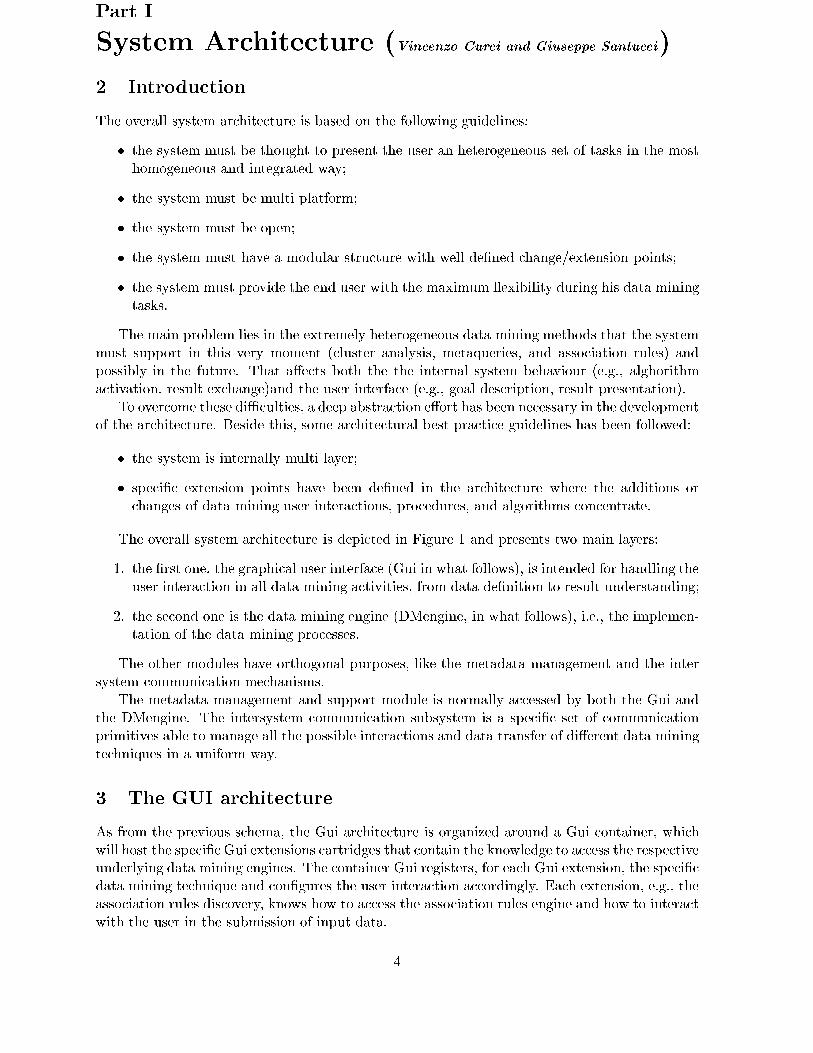
The overall system architecture is depicted in Figure 1 and presents two main layers:

1. the �rst one, the graphical user interface (Gui in what follows), is intended for handling the

user interaction in all data mining activities, from data de�nition to result understanding;

2. the second one is the data mining engine (DMengine, in what follows), i.e., the implemen-

tation of the data mining processes.

The other modules have orthogonal purposes, like the metadata management and the inter

system communication mechanisms.

The metadata management and support module is normally accessed by both the Gui and

the DMengine. The intersystem communication subsystem is a speci�c set of communication

primitives able to manage all the possible interactions and data transfer of di�erent data mining

techniques in a uniform way.

3 The GUI architecture

As from the previous schema, the Gui architecture is organized around a Gui container, which

will host the speci�c Gui extensions cartridges that contain the knowledge to access the respective

underlying data mining engines. The container Gui registers, for each Gui extension, the speci�c

data mining technique and con�gures the user interaction accordingly. Each extension, e.g., the

association rules discovery, knows how to access the association rules engine and how to interact

with the user in the submission of input data.

4

Database on analisys

ContainerGui

MQ Gui

Cluster Gui

Rule Gui

Abstract Dm

Engine

MQ Engine

Cluster Engine

Rules Engine

MetaData Support

Dm Persistence

Support

Main DM System Architecture

Figure 1: The overall system architecture

Summarizing, the Gui container gives the data mining system a common set of services, both

infrastructural and end user oriented.

The infrastructural services are:

� to register extensions, each of them implementing a speci�c interaction contract;

� to load on the Gui the speci�c extension options/commands;

� to route user commands to the active extension;

� to allow the user to select and access new extensions;

� to add speci�c controls for input insertion and result management.

The general end user added value services are:

� to provide the user with uniform presentation of the elaboration phases;

� to give access to general services like: to save, start, stop, load, and see the progress of

data mining analysis.

The main characteristics of a Gui extension are:

� the extension implements a set of commands, that are loaded at runtime by the container

Gui and made available to the end user;

5

� the extension implements the speci�c input/output modalities of the underlying data min-

ing algorithm;

� the speci�c modalities can be added to the general pre-existing ones, or can substitute

part of them.

4 The Abstract DMengine architecture

The DMengine architecture is the real soul of the system. It is completely decoupled from

the presentation layer, but its internal structure shows a strong similarity with the one of the

container Gui:

� there are some global services available to every speci�c data mining engine;

� there is a general reference abstract model of the engine (a conceptual framework);

� there are speci�c implementations of the real engines based on the type of data mining

analysis to perform.

The global services are used by every engine implementation, and are relate to:

� metadata management;

� con�guration saving/restoring;

� data access and DB connection management;

� internal data interchange and intersystem communication;

� data reduction.

The DMengine reference model is structured around a basic set of concepts:

� the global dataset, that contains all the needed information to perform and apply a data

mining technique: data and metadata. Normally it will contain tables, �elds and join

metadata, along with the data itself. The internal structure of the engine has been kept

very simple, collapsing the two abstraction levels (data and metadata) in a single data

structure, to give ease and uniform access to only the needed data. Roughly speaking, a

dataset is a relational subschema;

� the command manager is the DMengine interface towards the Gui. It is the interpreter of

user commands coming from the Gui and manages the access to internal data structure.

It is the unique point of contact between the Gui (both the container and the extension

Gui) and the engine. Typical operations performed through the manager are, at a very

high abstraction level:

{ to de�ne the initial set of data to operate on;

{ to de�ne , if any, some initialization data on the data mining technique in use;

{ to de�ne, if necessary, some starting hypotheses on the data to be mined;

{ to apply the algorithm to discover data mining hypotheses;

{ to store the hypotheses;

{ to verify the hypotheses on the same or di�erent, data.

� the hypothesis veri�er that veri�es a set of hypotheses on a dataset. The veri�er gives a

more accurate feedback of the hypothesis validity on data;

6

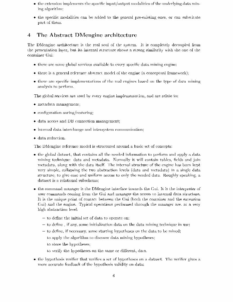
� the hypothesis discoverer, whose purpose is to discover hypotheses from the data, possibly

using hint hypotheses given directly by the user or as a result of a previous analysis.

� the data mining hypotheses that is the real piece of information the user needs from a data

mining analyses, whose content and format depends on the speci�c data mining algorithm

used.

Dm Engine Structure

Global DataSet

User Process Manager

Dm Discoverer

Dm Verificator

Hp 4

Hp 3

Hp 2

Hp 1

Datamining Hypotesis

This part must be specialised to implement specificdatamining technique

Figure 2: The data mining engine structure

4.1 General DMengine behavior

The general engine behavior is the following:

1. the user selects a dataset;

2. the user de�nes one or more data mining techniques to be applied on such a dataset;

3. possibly the user gives hints to the engine to drive the hypothesis search;

4. the user starts the engine, which use the discoverer to generate hypotheses that, in turn,

may be reanalyzed by the veri�er.

4.2 Speci�c DMengine implementation

The general DMengine behavior is an abstraction, which must be specialized by speci�c engines,

one for each available data mining method. So it is possible to envisage as many engines as the

7

di�erent techniques implemented by the system. The engines are made dynamically available

to the general engine framework and consequently to the user and are accessed through the

speci�c interaction Gui extension that must accompany each speci�c engine. The common

data structure used by all the specialized engines is the global dataset, which contains all the

information (data and metadata) needed by a data mining algorithm.

8

Part II

Visual Interface (Tiziana Catarci, Stephen Kimani, Giuseppe Santucci)

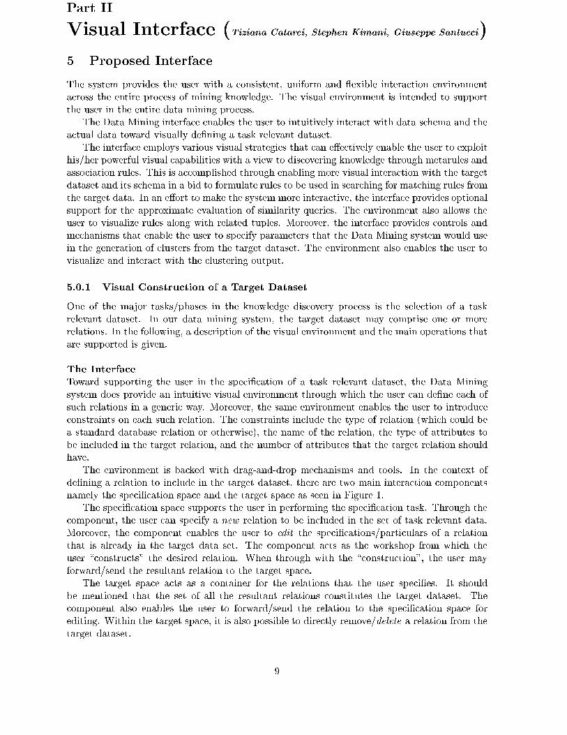
5 Proposed Interface

The system provides the user with a consistent, uniform and exible interaction environment

across the entire process of mining knowledge. The visual environment is intended to support

the user in the entire data mining process.

The Data Mining interface enables the user to intuitively interact with data schema and the

actual data toward visually de�ning a task relevant dataset.

The interface employs various visual strategies that can e�ectively enable the user to exploit

his/her powerful visual capabilities with a view to discovering knowledge through metarules and

association rules. This is accomplished through enabling more visual interaction with the target

dataset and its schema in a bid to formulate rules to be used in searching for matching rules from

the target data. In an e�ort to make the system more interactive, the interface provides optional

support for the approximate evaluation of similarity queries. The environment also allows the

user to visualize rules along with related tuples. Moreover, the interface provides controls and

mechanisms that enable the user to specify parameters that the Data Mining system would use

in the generation of clusters from the target dataset. The environment also enables the user to

visualize and interact with the clustering output.

5.0.1 Visual Construction of a Target Dataset

One of the major tasks/phases in the knowledge discovery process is the selection of a task

relevant dataset. In our data mining system, the target dataset may comprise one or more

relations. In the following, a description of the visual environment and the main operations that

are supported is given.

The Interface

Toward supporting the user in the speci�cation of a task relevant dataset, the Data Mining

system does provide an intuitive visual environment through which the user can de�ne each of

such relations in a generic way. Moreover, the same environment enables the user to introduce

constraints on each such relation. The constraints include the type of relation (which could be

a standard database relation or otherwise), the name of the relation, the type of attributes to

be included in the target relation, and the number of attributes that the target relation should

have.

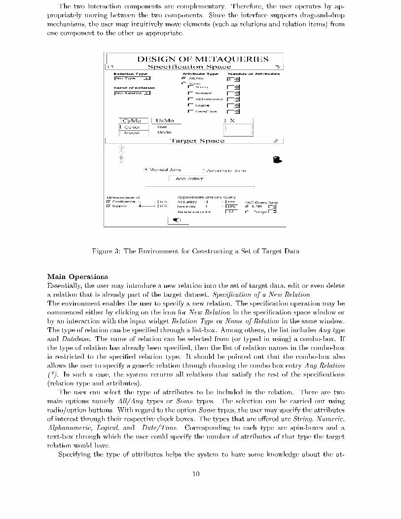
The environment is backed with drag-and-drop mechanisms and tools. In the context of

de�ning a relation to include in the target dataset, there are two main interaction components

namely the speci�cation space and the target space as seen in Figure 1.

The speci�cation space supports the user in performing the speci�cation task. Through the

component, the user can specify a new relation to be included in the set of task relevant data.

Moreover, the component enables the user to edit the speci�cations/particulars of a relation

that is already in the target data set. The component acts as the workshop from which the

user \constructs" the desired relation. When through with the \construction", the user may

forward/send the resultant relation to the target space.

The target space acts as a container for the relations that the user speci�es. It should

be mentioned that the set of all the resultant relations constitutes the target dataset. The

component also enables the user to forward/send the relation to the speci�cation space for

editing. Within the target space, it is also possible to directly remove/delete a relation from the

target dataset.

9

The two interaction components are complementary. Therefore, the user operates by ap-

propriately moving between the two components. Since the interface supports drag-and-drop

mechanisms, the user may intuitively move elements (such as relations and relation items) from

one component to the other as appropriate.

Figure 3: The Environment for Constructing a Set of Target Data

Main Operations

Essentially, the user may introduce a new relation into the set of target data, edit or even delete

a relation that is already part of the target dataset. Speci�cation of a New Relation

The environment enables the user to specify a new relation. The speci�cation operation may be

commenced either by clicking on the icon for New Relation in the speci�cation space window or

by an interaction with the input widget Relation Type or Name of Relation in the same window.

The type of relation can be speci�ed through a list-box. Among others, the list includesAny type

and Database. The name of relation can be selected from (or typed in using) a combo-box. If

the type of relation has already been speci�ed, then the list of relation names in the combo-box

is restricted to the speci�ed relation type. It should be pointed out that the combo-box also

allows the user to specify a generic relation through choosing the combo-box entry Any Relation

(*). In such a case, the system returns all relations that satisfy the rest of the speci�cations

(relation type and attributes).

The user can select the type of attributes to be included in the relation. There are two

main options namely All/Any types or Some types. The selection can be carried out using

radio/option buttons. With regard to the option Some types, the user may specify the attributes

of interest through their respective check boxes. The types that are o�ered are String, Numeric,

Alphanumeric, Logical, and Date/Time. Corresponding to each type are spin-boxes and a

text-box through which the user could specify the number of attributes of that type the target

relation would have.

Specifying the type of attributes helps the system to have some knowledge about the at-

10

tributes that are of interest to the user. However, given that the user might also have input

the number of attributes, there is a possibility that the system might not be able to �gure out

which attributes, of the type that was speci�ed, to include or to leave out. To address this

complication, the interface o�ers the user the freedom to decide which attributes to include and

in what order. Fundamentally, the system renders this through the generation of \resource"

relation(s) and a \skeleton" relation, which it puts in the speci�cation space.

\Resource" relation(s) are relations of the speci�ed relation type and attribute types. Each

such relation has a handle corresponding to the relation's name (upper handle). Moreover, each

of the relation's attributes has a handle (attribute handle). The \skeleton" relation is a blank

relation which the user works on as s/he desires. \Resource" relations act as the resource from

which the user gets the materials for building the \skeleton" relation. The \skeleton" relation

provides the structure/skeleton on which the user builds a target relation.

The \skeleton" relation comes with a name and with slots into which attributes can be

slotted in. If there are multiple \resource" relations, then the \skeleton" relation takes on a

generic name. In the case where there is only one \resource" relation, then the \skeleton"

relation acquires a name similar to the \resource" relation. Figure 1 shows the environment

with multiple \resource" relations and a \skeleton" relation that has a generic name (X ).

The number of slots corresponds to the number of attributes that was speci�ed. If the

number that was speci�ed is greater than the actual number of attributes, then the system

uses the actual number of attributes and generates a corresponding number of slots. Like the

\resource" relations, the \skeleton" relation also has a handle corresponding to the name (upper

handle). Moreover, each slot that has been �lled with an attribute also has a handle (attribute

handles). It is worth mentioning that in the environment the user can hold/pick and drag a

relation's name by the upper handle and an attribute by the attribute handle, using the hand

tool.

In the case where there are multiple \resource" relations, the user may pick and drag an

attribute from any of the relations and slot it in where s/he wants in the \skeleton" relation.

If the user would like to use attributes only from one of the multiple \resource" relations,

s/he could pick the relation's upper handle (relation's name) and overlay it on the \skeleton"

relation's name. The operation sets up the \skeleton" relation to receive attributes only from the

one \resource" relation of interest. As for the case where there is only one \resource" relation,

the user may drag attributes from the relation and insert them into the \skeleton" relation's

slots in a straightforward manner.

The user may also drag attributes up and down (rearranging the attributes) in the \skeleton"

relation itself. The user uses the hand tool to hold the attribute handles thereby picking the

respective attributes and therefore s/he can move the attributes up and down as s/he wishes.

When dealing with multiple \resource" relations, it is possible to delete or change a name

that the user may have assigned to the \skeleton" relation. To delete the relation's name, the

user selects the hand tool, uses the tool to pick the name by its handle and drops the name into

the trash-bin or presses the delete key. Alternatively, the user may select the name by using

the pointer tool and then press the delete key. The immediate result of the deletion is that the

\skeleton" relation assumes a generic name. With regard to changing the name of the \skeleton"

relation, the user may drag another relation's name from the pool of \resource" relations and

overlay the current \skeleton" relation's name with the new name.

The user may also delete an attribute from the \skeleton" relation. Toward that, the user

picks the attribute by its handle and drops it into the trash-bin or presses the delete key. The

same operation can be accomplished by selecting the attribute using the pointer tool and then

pressing the delete key.

Once the user is satis�ed with the \skeleton" relation s/he has built, s/he may forward it

to the target space. This indicates that the relation becomes part of the target dataset. The

forwarding may be accomplished either by drag and drop or by iconic commands. With respect

11

to drag and drop approach, the hand tool can be used to hold the (\skeleton") relation's upper

handle. Then the user can drag the relation and drop it into the target space. In regard to iconic

commands, the user selects the pointer tool, clicks the upper handle and clicks the icon for To

Target Space. The interface gets ready for another task e.g. speci�cation of another new relation.

Editing a Relation

The user can edit a relation that is already in the target space. With the hand tool, the user

holds the relation of interest by the upper handle, drags the relation and drops it into the spec-

i�cation space. As an alternative, the user may pick the pointer tool, click the upper handle of

the relation of interest, and then click on the icon for To Speci�cation Space in the target space

window. This causes the relation to be made available in the speci�cation space for editing.

Once the relation of interest gets back to the speci�cation space, the interface gets updated

to support the anticipated editing. The relation of interest becomes the \skeleton" relation with

\delicate" (subject-to- change) attributes. The system reloads the respective speci�cations and

\resource" relation(s). At this level, editing operations then resemble the speci�cation opera-

tions in the previous discussion on Speci�cation of a New Relation.

Deleting a Relation

The user can delete/remove a relation from the target space. With the hand tool, the user holds

the relation of interest by using the relation's upper handle. The user then drags the relation

and drops it in the trash-bin or presses the delete key. Alternatively, the user could accomplish

the same by using the pointer tool and the delete key. The user selects the pointer tool. With

the tool, the user clicks the upper handle of the relation of interest. This causes the relation to

be selected. With the relation selected, the user presses the delete key.

It is important to keep in mind that all the mentioned relation operations do not a�ect the

original relations/data in any way. The operations de�ne the set of data that is of interest to

the user for the data mining task at hand.

5.1 Approximate Similarity Queries

In order to make the data mining more interactive, the interface provides an optional avenue

through which the user can specify approximate similarity queries.

Parameter Speci�cation

The system provides support for approximate similarity queries across all the implementations

of data mining strategies. In the each of the environments, the input widgets for similarity

query parameters are placed just below where the input widgets for the other data mining

strategy-speci�c parameters are placed.

It is worth mentioning that approximate similarity query support is especially useful where

clustering inputs or outputs are involved.

In [6, Part III], PAC queries are proposed as a search paradigm for quality-controlled ap-

proximate similarity search. In particular, PAC (range and k-NN) queries allow the error on

the query result to exceed a certain threshold (indicated by an accuracy parameter �) with a

probability not higher than the value of the reliability parameter Æ. In order to perform a PAC

query, the user has therefore to specify a value for the accuracy and the reliability parameters �

and Æ. The environment provides two sliders to adjust the values of both accuracy and reliabil-

ity parameters from a maximum of 100% (exact query) to a minimum application-speci�c value

(e.g. 50% for both parameters).

Each similarity query requires a reference point to be expressed. The interface provides a

text-box through which the coordinates of the reference point may be input. When the user

clicks inside the text-box, the \coordinate selector" tool in the output window blinks. It should

12

be pointed out that blinking occurs only when there is already some visualization of results. The

user may simply type in the text-box the coordinate values of a reference point thereby causing

the blinking to stop. Alternatively, the user may move to the output window and directly click

the point of interest. The blinking stops and the values of the clicked point get automatically

recorded in the Reference point input widget. In the latter way of specifying the reference point,

the user relies on the visualization of results from previous data mining tasks. In particular,

since results of clustering are more likely to be used than those of meta-querying or association

rules, the supposition is that the output window is the scatter plot of the Overview + Details

visualization of clusters. The foregoing visualization is discussed later in this Section under

Visualizing Clustering Output within the clustering environment.

The last parameter requested by a PAC query is dependent on the query type. In particular,

for k-NN queries the user has to specify the number k of requested result, whereas for range

queries the user �xes the distance threshold that points in the result should not exceed. The

interface provides a spin-box and an alternate text-box for each of the two values. As for the

query type, the interface o�ers two radio buttons that allow the user to specify either k-NN

type or Range type. Moreover, selecting a query type activates the corresponding text-box and

spin-box. Upon clicking the radio button for k-NN, the user may directly type in the value of

k or use the spin-box. On the hand, when the user selects the radio button for Range or clicks

inside the respective and already activated text-box, the \circle drawing" tool in the output

window blinks. In a manner similar to the interactive speci�cation of a reference point, blinking

occurs only when there is already some output from previous data mining tasks. The user may

manually enter the query radius in the text-box or use the spin-box. The speci�cation causes

the blinking to stop. Alternatively, the user may specify the radius by dragging within the

output window, which is essentially the scatter plot of clusters. The dragging operation causes

a circle to be drawn on the scatter plot with the respective radius being dynamically re ected in

the text-box. When satis�ed with the radius of the circle instance, the user releases the mouse

button. The radius gets recorded in the text-box as the query radius and the blinking stops.

It should be mentioned that the user can always interrupt or even cancel an interactive

speci�cation process by clicking anywhere outside the context of the process or by simply pressing

the escape key.

The \torch" icon is used to instruct the underlying system to actually perform the PAC

query on the target dataset based on the speci�ed approximate similarity query parameters

(and data mining strategy-speci�c parameters).

5.2 Metaqueries

In the following, a discussion on how the system supports the formulation of metaqueries and

visualization of metaquery results is given.

Designing Metaqueries

Pattern Formulation

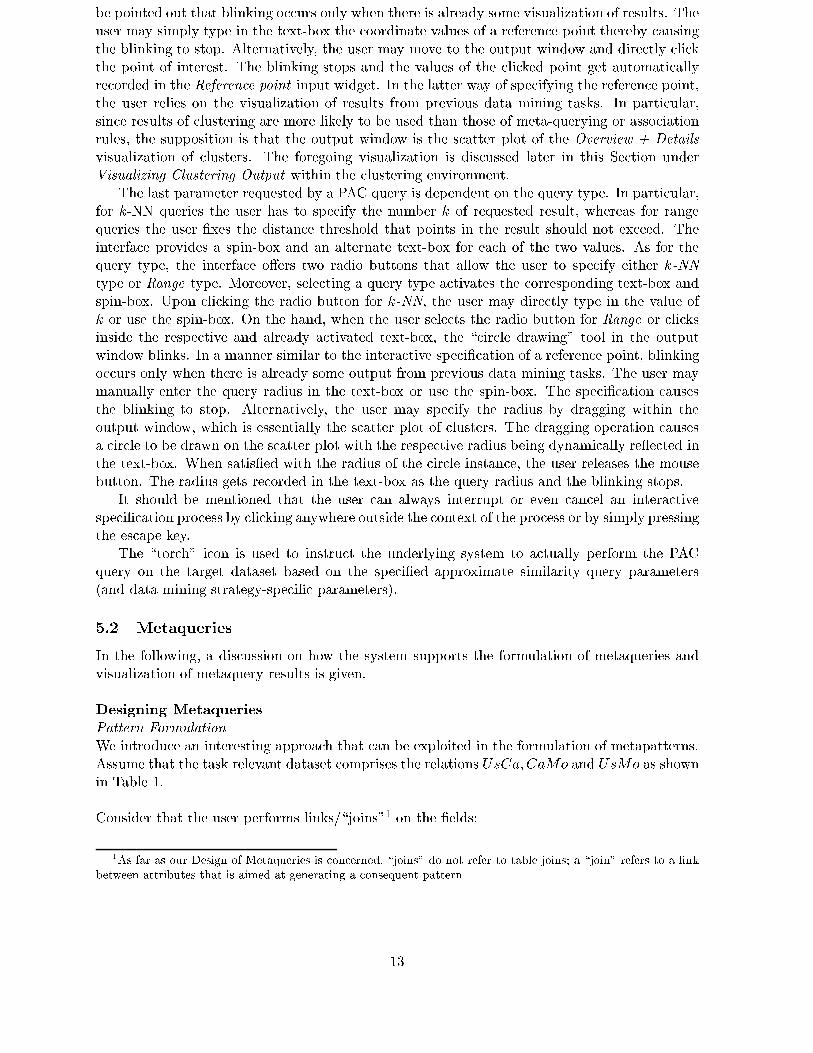
We introduce an interesting approach that can be exploited in the formulation of metapatterns.

Assume that the task relevant dataset comprises the relations UsCa;CaMo and UsMo as shown

in Table 1.

Consider that the user performs links/\joins"1 on the �elds:

1As far as our Design of Metaqueries is concerned, \joins" do not refer to table joins; a \join" refers to a link

between attributes that is aimed at generating a consequent pattern

13

UsCa

User Carrier

John K. Omnitel

John K. Tim

Anastasia A. Omnitel

CaMo

Carrier Model

Tim Nokia

Omnitel Siemens

Wind Nokia

UsMo

User Model

John K. Siemens

John K. Nokia

Anastasia A. Siemens

Table 1: The Task Relevant Dataset

UsMo:User and UsCa:User

UsMo:Model and CaMo:Model

UsCa:Carrier and CaMo:Carrier

with constraints:

UsMo:User and UsCa:User = \JohnK:00

UsMo:Model and CaMo:Model = \Nokia00

Having linked the �elds, we have the following:

UsMo(User;Model); UsCa(User; Carrier); CaMo(Carrier;Model)

Introducing the constraints, we get:

UsMo(\JohnK:00; \Nokia00); UsCa(\JohnK:00; Carrier);

CaMo(Carrier; \Nokia00)

which resembles:

R(x; z); P (x; y); Q(y; z)

where P;Q;R are relations and x; y; z are attributes or literal values.

Intuitively, there appears to be a general transitive pattern/rule of the form:

R(x; z) P (x; y); Q(y; z)

In fact the pattern is a metaquery. Therefore, from the discussion, a possible instantiation

� of the metaquery is such that:

� =< R(x; z); UsMo(\JohnK:00 ; \Nokia00) >;< P (x; y);

UsCa(\JohnK:00; Carrier) >;< Q(y; z); CaMo(Carrier; \Nokia00) >

and thus the following horn rule:

UsMo(\JohnK:00; \Nokia00) UsCa(\JohnK:00; Carrier);

CaMo(Carrier; \Nokia00)

The Metaquery Environment

Consider that the user visually constructs a task relevant dataset2 thereby de�ning a dataset

2The construction refers to the approach that was described earlier in the section on Visual Construction of a

Task Relevant Dataset

14

consisting of the relations in Table 1.

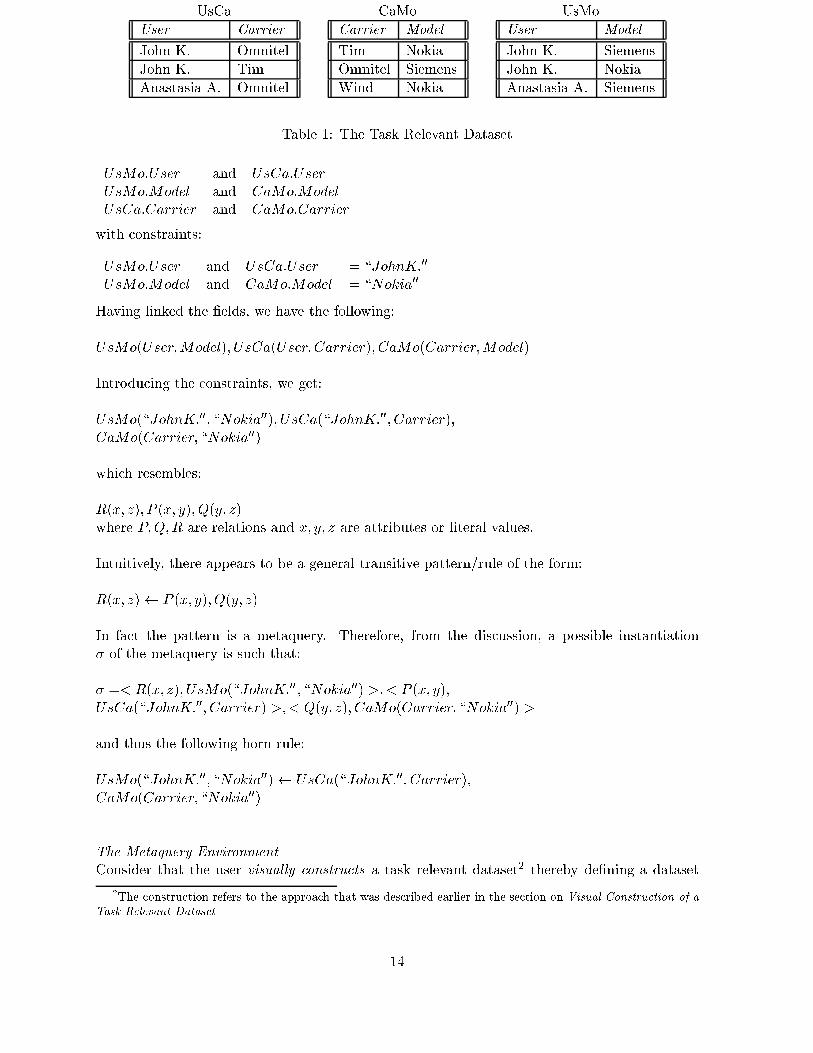
Figure 4: The Environment for Formulating Metaqueries

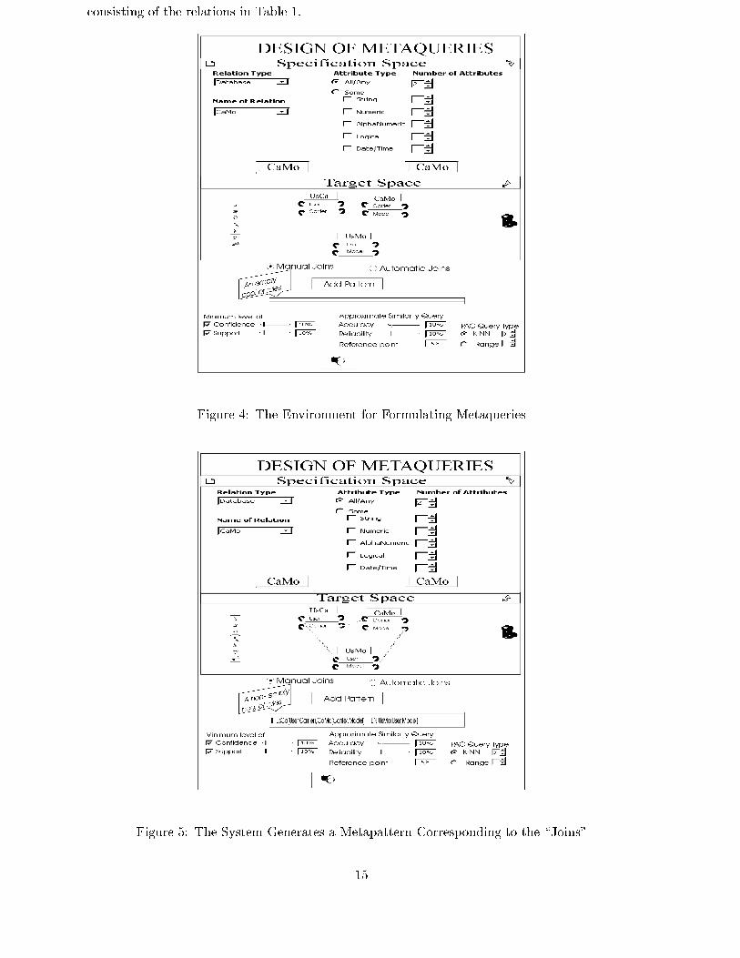
Figure 5: The System Generates a Metapattern Corresponding to the \Joins"

15

The Design of Metaqueries environment enables the user to either de�ne links/\joins" man-

ually (Manual Joins) or have them de�ned automatically by the system (Automatic Joins) by

selecting the relevant option button.

In the automated option, the user does not need to perform any linking operation. The

system automatically analyses the metadata of the relations for any possible or applicable

links/connections. The user may proceed and click the \Add Pattern" command button to

have the system generate metapatterns that correspond to the links. The system puts the

metapatterns into some \pool" (of metaqueries) located just below the command button.

As regards the manual speci�cation of links, the user selects an attribute of interest by using

its \hook". The operation is realized through the use of the mouse-pointer or the \pointer"

tool. The operation causes the \join" tool to blink, demanding attention. The user picks the

\join" tool from the tool-box causing the tool to stop blinking. The relations blink, demanding

attention. With the \join" tool, the user selects an attribute (by its \hook") of another relation

causing the relations to stop blinking. The two attributes (\hooks") get linked/connected with

some \chain". An alternative way of accomplishing the linking operation is by using the \hand"

tool. In this case, the user selects the \hand" tool from the tool-box, causing the relations to

blink. The user uses the \hand" tool to hold attribute of interest (by its \hook"). The user

drags and drops it on the \hook" of an attribute of another relation causing the relations to

stop blinking. The two respective attributes get connected with a \chain".

The environment also o�ers mechanisms for introducing constraints on the linked �elds. The

user selects a de�ned link/connection by using the mouse-pointer or the \pointer" tool. The

\disconnect" and \edit" tools blink, demanding attention. The user picks the \edit" tool from

the tool-box causing the \disconnect" and \edit" tools to stop blinking. The selected connection

provides some combo-box through which the user may type in some constraint or get a list of

attribute values to select from. Entering or clicking anywhere else causes the combo-box inputs

to be taken. An optional way of introducing a (or editing the) constraint is by double-clicking

the respective connection (or de�ned constraint).

The user may wish to delete a de�ned connection or constraint. In regard to deleting a

de�ned connection, the user selects it by using the mouse-pointer or the \pointer" tool. The

\disconnect" and \edit" tools blink. The user either picks the \disconnect" tool from the

tool-box or simply presses the delete key. The \disconnect" and \edit" tools stop blinking. The

connection of interest gets broken. With respect to deleting a de�ned constraint, the user selects

it thereby causing the \delete" and \edit" tools to blink. The user either picks the \delete" tool

from the tool-box or presses the delete key. The \delete" and \edit" tools stop blinking. The

constraint that was selected gets deleted. It should be mentioned that a more intuitive and

straightforward way of deleting a connection or constraint is by holding, dragging, and dropping

it in the trash-bin.

Figure 2 shows the initial status of the interface with the task relevant dataset.

When satis�ed with the links/\joins" de�ned, the user may instruct the system to generate

a metapattern (Add Pattern) corresponding to the links. It should be pointed out that, at this

point, the system does not need to use/search the database. At the current level of operation, the

generation of a metapattern is simply an analysis that relies only on metadata and link/\join"

information. The generated pattern is put in a pool. The user may repeat the same process

for the design of another or other metapatterns. It can be observed that the user has \direct"

interaction with the target data and also has \direct" control over the metapatterns that are

put in the pool. The patterns in the pool constitute a major parameter of the query that will

be used to search for speci�c rules in the database corresponding to the patterns. Consider that

the user introduces the links:UsMo:User and UsCa:User

UsMo:Model and CaMo:Model

UsCa:Carrier and CaMo:Carrier

16

Assuming that the user is satis�ed with the \joins", and instructs the system to generate a

corresponding metapattern, Figure 3 shows the interface at the current level of operation.

The user may also specify the threshold values for con�dence and support measures. There

are sliders and text-boxes to support the speci�cation. Moreover, the user may specify the

approximate similarity query parameters. The user may instruct the system to search for spe-

ci�c rules from the dataset that correspond to the metapatterns in the pool and that satisfy

the speci�ed threshold levels, by clicking the \torch" icon. The system returns the obtained

metarules and provides various visualizations for the same. It should be mentioned that the

system supports dynamic \updates" in that any subsequent changes to the metaquerying pa-

rameters are directly re ected in the visualization(s). Consequently, the user does not need to

click the \torch" icon every time the parameters are changed. The dynamic functionality holds

as long as the target dataset has not been modi�ed.

Visualizing Metaqueries

The system provides visualizations for the metarules that are obtained from the dataset. For

any metarule, the parameters that are of principal interest are:

� Measures of interestingness (such as con�dence and support)

� Relationship/association between the head part and the body part

� Number of items participating in the rule (total number in the rule; number in the head,

number in the body)

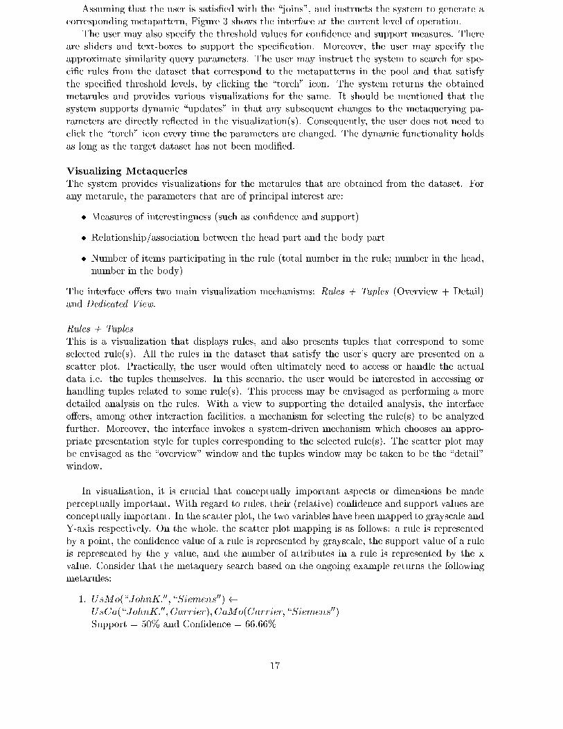
The interface o�ers two main visualization mechanisms: Rules + Tuples (Overview + Detail)

and Dedicated View.

Rules + Tuples

This is a visualization that displays rules, and also presents tuples that correspond to some

selected rule(s). All the rules in the dataset that satisfy the user's query are presented on a

scatter plot. Practically, the user would often ultimately need to access or handle the actual

data i.e. the tuples themselves. In this scenario, the user would be interested in accessing or

handling tuples related to some rule(s). This process may be envisaged as performing a more

detailed analysis on the rules. With a view to supporting the detailed analysis, the interface

o�ers, among other interaction facilities, a mechanism for selecting the rule(s) to be analyzed

further. Moreover, the interface invokes a system-driven mechanism which chooses an appro-

priate presentation style for tuples corresponding to the selected rule(s). The scatter plot may

be envisaged as the \overview" window and the tuples window may be taken to be the \detail"

window.

In visualization, it is crucial that conceptually important aspects or dimensions be made

perceptually important. With regard to rules, their (relative) con�dence and support values are

conceptually important. In the scatter plot, the two variables have been mapped to grayscale and

Y-axis respectively. On the whole, the scatter plot mapping is as follows: a rule is represented

by a point, the con�dence value of a rule is represented by grayscale, the support value of a rule

is represented by the y value, and the number of attributes in a rule is represented by the x

value. Consider that the metaquery search based on the ongoing example returns the following

metarules:

1. UsMo(\JohnK:00; \Siemens00)

UsCa(\JohnK:00; Carrier); CaMo(Carrier; \Siemens00)

Support = 50% and Con�dence = 66.66%

17

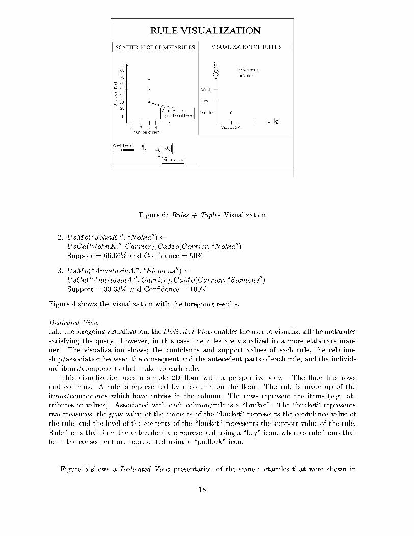
Figure 6: Rules + Tuples Visualization

2. UsMo(\JohnK:00; \Nokia00)

UsCa(\JohnK:00; Carrier); CaMo(Carrier; \Nokia00)

Support = 66.66% and Con�dence = 50%

3. UsMo(\AnastasiaA:"; \Siemens00)

UsCa(\AnastasiaA:00; Carrier); CaMo(Carrier; \Siemens00)

Support = 33.33% and Con�dence = 100%

Figure 4 shows the visualization with the foregoing results.

Dedicated View

Like the foregoing visualization, theDedicated View enables the user to visualize all the metarules

satisfying the query. However, in this case the rules are visualized in a more elaborate man-

ner. The visualization shows; the con�dence and support values of each rule, the relation-

ship/association between the consequent and the antecedent parts of each rule, and the individ-

ual items/components that make up each rule.

This visualization uses a simple 2D oor with a perspective view. The oor has rows

and columns. A rule is represented by a column on the oor. The rule is made up of the

items/components which have entries in the column. The rows represent the items (e.g. at-

tributes or values). Associated with each column/rule is a \bucket". The \bucket" represents

two measures; the gray value of the contents of the \bucket" represents the con�dence value of

the rule, and the level of the contents of the \bucket" represents the support value of the rule.

Rule items that form the antecedent are represented using a \key" icon, whereas rule items that

form the consequent are represented using a \padlock" icon.

Figure 5 shows a Dedicated View presentation of the same metarules that were shown in

18

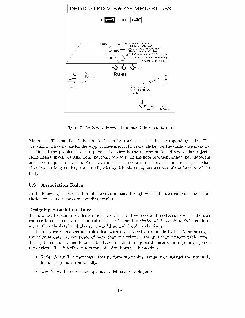
Figure 7: Dedicated View : Elaborate Rule Visualization

Figure 4. The handle of the \bucket" can be used to select the corresponding rule. The

visualization has a scale for the support measure, and a grayscale key for the con�dence measure.

One of the problems with a perspective view is the determination of size of far objects.

Nonetheless, in our visualization, the icons/\objects" on the oor represent either the antecedent

or the consequent of a rule. As such, their size is not a major issue in interpreting the visu-

alization; as long as they are visually distinguishable as representations of the head or of the

body.

5.3 Association Rules

In the following is a description of the environment through which the user can construct asso-

ciation rules and view corresponding results.

Designing Association Rules

The proposed system provides an interface with intuitive tools and mechanisms which the user

can use to construct association rules. In particular, the Design of Association Rules environ-

ment o�ers \baskets" and also supports \drag and drop" mechanisms.

In most cases, association rules deal with data stored on a single table. Nonetheless, if

the relevant data are composed of more than one relation, the user may perform table joins3.

The system should generate one table based on the table joins the user de�nes (a single joined

table/view). The interface caters for both situations i.e. it provides:

� De�ne Joins: The user may either perform table joins manually or instruct the system to

de�ne the joins automatically.

� Skip Joins: The user may opt not to de�ne any table joins.

19

OrdProd

OrderID ProdID

121 P002

121 P003

122 P004

123 P001

123 P004

124 P003

125 P001

126 P001

126 P005

Product

ProdID ProdName

P001 Shirt

P002 Shoes

P003 Socks

P004 Sweater

P005 Tie

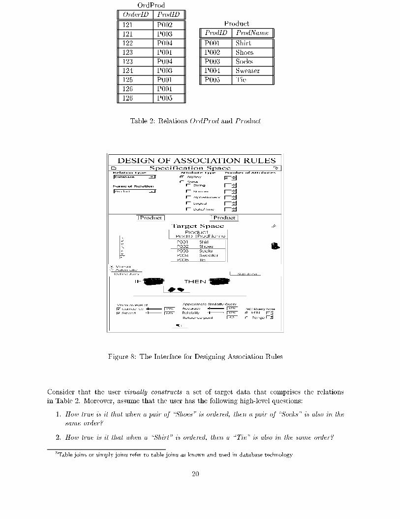
Table 2: Relations OrdProd and Product

Figure 8: The Interface for Designing Association Rules

Consider that the user visually constructs a set of target data that comprises the relations

in Table 2. Moreover, assume that the user has the following high-level questions:

1. How true is it that when a pair of \Shoes" is ordered, then a pair of \Socks" is also in the

same order?

2. How true is it that when a \Shirt" is ordered, then a \Tie" is also in the same order?

3Table joins or simply joins refer to table joins as known and used in database technology

20

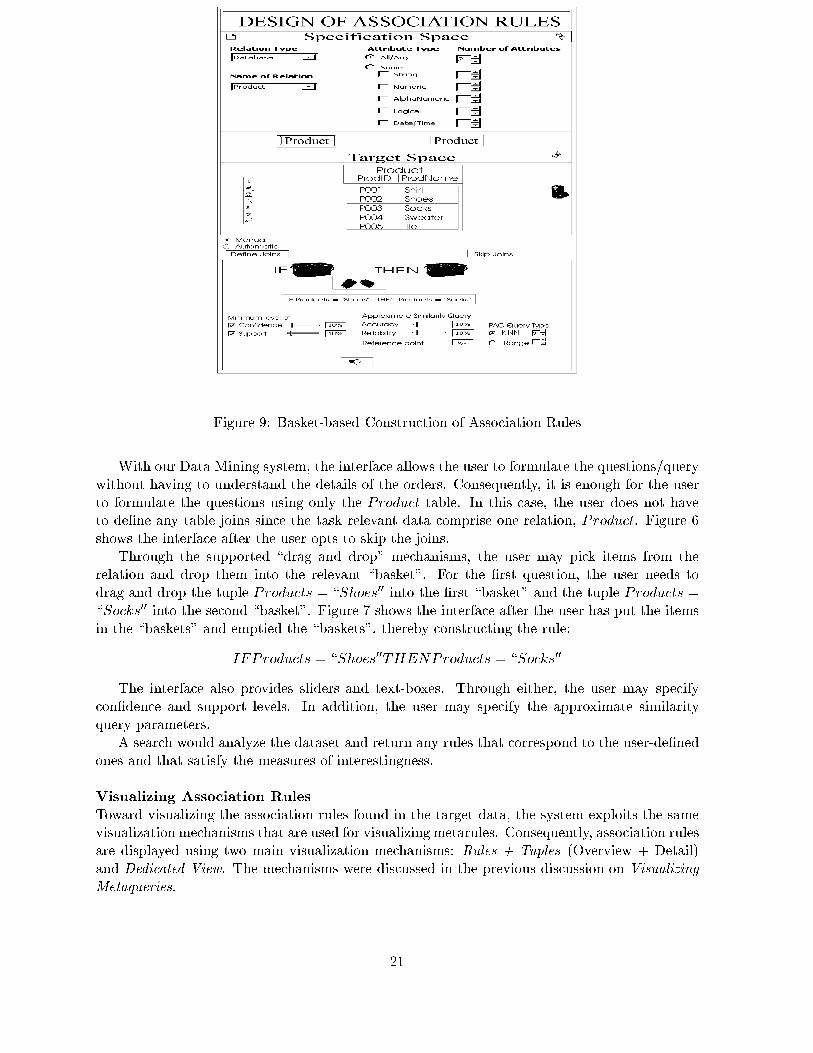
Figure 9: Basket-based Construction of Association Rules

With our Data Mining system, the interface allows the user to formulate the questions/query

without having to understand the details of the orders. Consequently, it is enough for the user

to formulate the questions using only the Product table. In this case, the user does not have

to de�ne any table joins since the task relevant data comprise one relation, Product. Figure 6

shows the interface after the user opts to skip the joins.

Through the supported \drag and drop" mechanisms, the user may pick items from the

relation and drop them into the relevant \basket". For the �rst question, the user needs to

drag and drop the tuple Products = \Shoes00 into the �rst \basket" and the tuple Products =

\Socks00 into the second \basket". Figure 7 shows the interface after the user has put the items

in the \baskets" and emptied the \baskets", thereby constructing the rule:

IFProducts = \Shoes00THENProducts = \Socks00

The interface also provides sliders and text-boxes. Through either, the user may specify

con�dence and support levels. In addition, the user may specify the approximate similarity

query parameters.

A search would analyze the dataset and return any rules that correspond to the user-de�ned

ones and that satisfy the measures of interestingness.

Visualizing Association Rules

Toward visualizing the association rules found in the target data, the system exploits the same

visualization mechanisms that are used for visualizing metarules. Consequently, association rules

are displayed using two main visualization mechanisms: Rules + Tuples (Overview + Detail)

and Dedicated View. The mechanisms were discussed in the previous discussion on Visualizing

Metaqueries.

21

5.4 Clustering

The clustering environment does provide controls and mechanisms that enable the user to specify

parameters that the Data Mining system would use in the generation of clusters from the target

dataset. Moreover, the environment also enables the user to visualize and interact with various

clustering results.

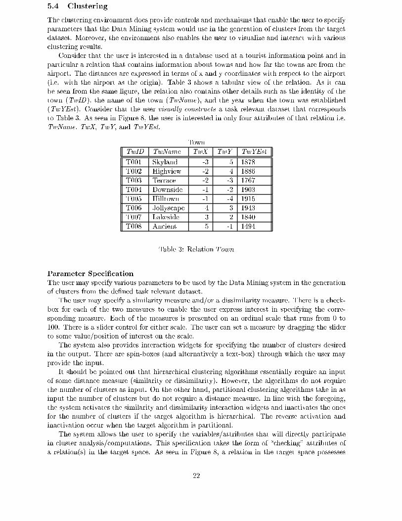
Consider that the user is interested in a database used at a tourist information point and in

particular a relation that contains information about towns and how far the towns are from the

airport. The distances are expressed in terms of x and y coordinates with respect to the airport

(i.e. with the airport as the origin). Table 3 shows a tabular view of the relation. As it can

be seen from the same �gure, the relation also contains other details such as the identity of the

town (TwID), the name of the town (TwName), and the year when the town was established

(TwYEst). Consider that the user visually constructs a task relevant dataset that corresponds

to Table 3. As seen in Figure 8, the user is interested in only four attributes of that relation i.e.

TwName, TwX, TwY, and TwYEst.

Town

TwID TwName TwX TwY TwYEst

T001 Skyland -3 5 1878

T002 Highview -2 4 1886

T003 Terrace -2 -3 1767

T004 Downside -1 -2 1903

T005 Hilltown -1 -4 1915

T006 Jollyscape 4 3 1943

T007 Lakeside 3 2 1840

T008 Ancient 5 -1 1494

Table 3: Relation Town


The user may specify various parameters to be used by the Data Mining system in the generation

of clusters from the de�ned task relevant dataset.

The user may specify a similarity measure and/or a dissimilarity measure. There is a check-

box for each of the two measures to enable the user express interest in specifying the corre-

sponding measure. Each of the measures is presented on an ordinal scale that runs from 0 to

100. There is a slider control for either scale. The user can set a measure by dragging the slider

to some value/position of interest on the scale.

The system also provides interaction widgets for specifying the number of clusters desired

in the output. There are spin-boxes (and alternatively a text-box) through which the user may

provide the input.

It should be pointed out that hierarchical clustering algorithms essentially require an input

of some distance measure (similarity or dissimilarity). However, the algorithms do not require

the number of clusters as input. On the other hand, partitional clustering algorithms take in as

input the number of clusters but do not require a distance measure. In line with the foregoing,

the system activates the similarity and dissimilarity interaction widgets and inactivates the ones

for the number of clusters if the target algorithm is hierarchical. The reverse activation and

inactivation occur when the target algorithm is partitional.

The system allows the user to specify the variables/attributes that will directly participate

in cluster analysis/computations. This speci�cation takes the form of \checking" attributes of

a relation(s) in the target space. As seen in Figure 8, a relation in the target space possesses

22

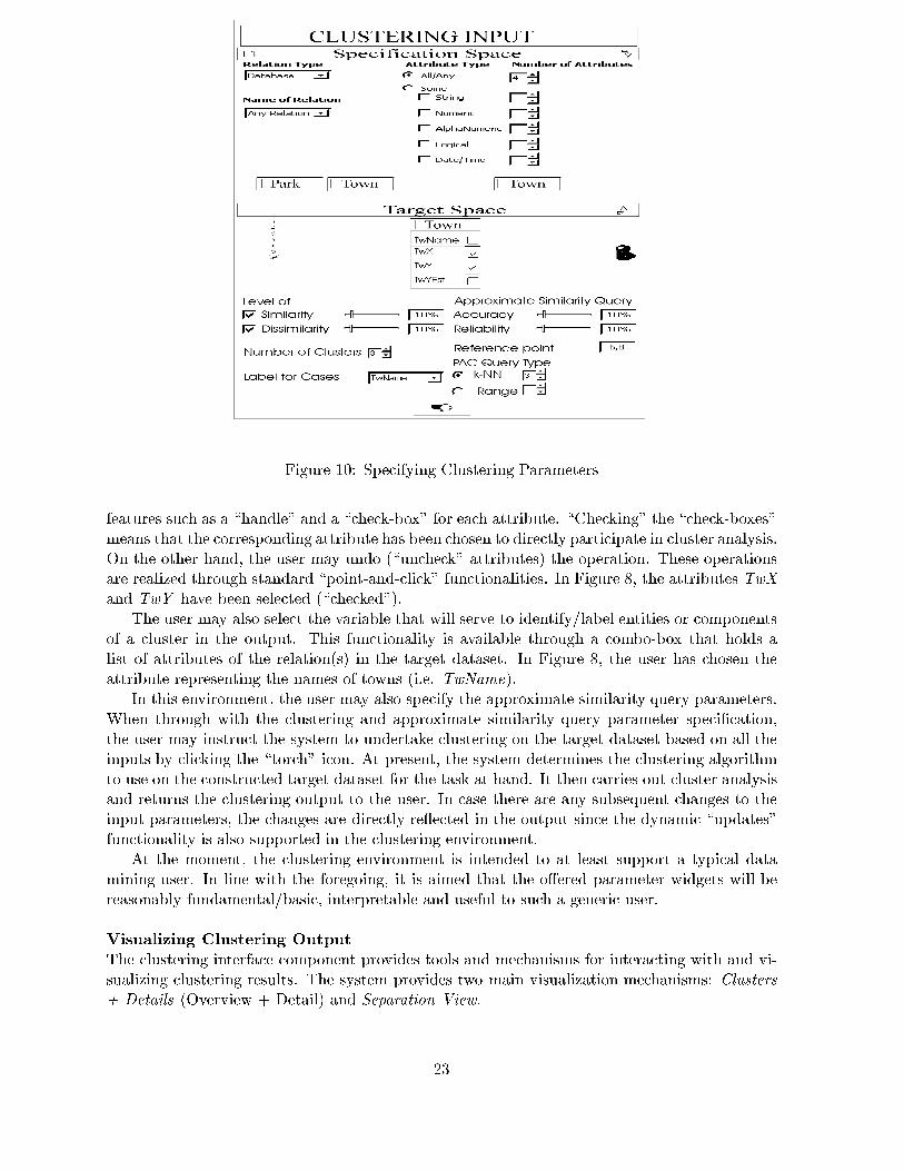
Figure 10: Specifying Clustering Parameters

features such as a \handle" and a \check-box" for each attribute. \Checking" the \check-boxes"

means that the corresponding attribute has been chosen to directly participate in cluster analysis.

On the other hand, the user may undo (\uncheck" attributes) the operation. These operations

are realized through standard \point-and-click" functionalities. In Figure 8, the attributes TwX

and TwY have been selected (\checked").

The user may also select the variable that will serve to identify/label entities or components

of a cluster in the output. This functionality is available through a combo-box that holds a

list of attributes of the relation(s) in the target dataset. In Figure 8, the user has chosen the

attribute representing the names of towns (i.e. TwName).

In this environment, the user may also specify the approximate similarity query parameters.

When through with the clustering and approximate similarity query parameter speci�cation,

the user may instruct the system to undertake clustering on the target dataset based on all the

inputs by clicking the \torch" icon. At present, the system determines the clustering algorithm

to use on the constructed target dataset for the task at hand. It then carries out cluster analysis

and returns the clustering output to the user. In case there are any subsequent changes to the

input parameters, the changes are directly re ected in the output since the dynamic \updates"

functionality is also supported in the clustering environment.

At the moment, the clustering environment is intended to at least support a typical data

mining user. In line with the foregoing, it is aimed that the o�ered parameter widgets will be

reasonably fundamental/basic, interpretable and useful to such a generic user.

Visualizing Clustering Output

The clustering interface component provides tools and mechanisms for interacting with and vi-

sualizing clustering results. The system provides two main visualization mechanisms: Clusters

+ Details (Overview + Detail) and Separation View.

23

CLUSTERING OUTPUT

Cluster quality

Standard Tools

Selected point and thus

the outline around it

DETAILSCLUSTERS

Hilltown is a town

It is located 4.12 miles

South West of the airport

It was established in 1915 AD

HILLTOWN

SEPARATION OF THE CLUSTER FROM THE OTHERS

Cluster1 Cluster2 Outlier1

Separa

tion

Cluster quality Cluster density

Standard visualization

and sorting tools

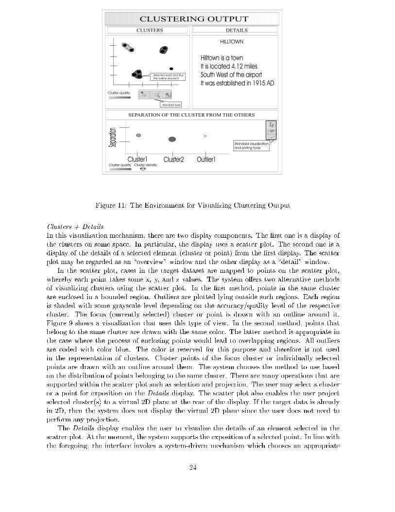
Figure 11: The Environment for Visualizing Clustering Output

Clusters + Details

In this visualization mechanism, there are two display components. The �rst one is a display of

the clusters on some space. In particular, the display uses a scatter plot. The second one is a

display of the details of a selected element (cluster or point) from the �rst display. The scatter

plot may be regarded as an \overview" window and the other display as a \detail" window.

In the scatter plot, cases in the target dataset are mapped to points on the scatter plot,

whereby each point takes some x, y, and z values. The system o�ers two alternative methods

of visualizing clusters using the scatter plot. In the �rst method, points in the same cluster

are enclosed in a bounded region. Outliers are plotted lying outside such regions. Each region

is shaded with some grayscale level depending on the accuracy/quality level of the respective

cluster. The focus (currently selected) cluster or point is drawn with an outline around it.

Figure 9 shows a visualization that uses this type of view. In the second method, points that

belong to the same cluster are drawn with the same color. The latter method is appropriate in

the case where the process of enclosing points would lead to overlapping regions. All outliers

are coded with color blue. The color is reserved for this purpose and therefore is not used

in the representation of clusters. Cluster points of the focus cluster or individually selected

points are drawn with an outline around them. The system chooses the method to use based

on the distribution of points belonging to the same cluster. There are many operations that are

supported within the scatter plot such as selection and projection. The user may select a cluster

or a point for exposition on the Details display. The scatter plot also enables the user project

selected cluster(s) to a virtual 2D plane at the rear of the display. If the target data is already

in 2D, then the system does not display the virtual 2D plane since the user does not need to

perform any projection.

The Details display enables the user to visualize the details of an element selected in the

scatter plot. At the moment, the system supports the exposition of a selected point. In line with

the foregoing, the interface invokes a system-driven mechanism which chooses an appropriate

24

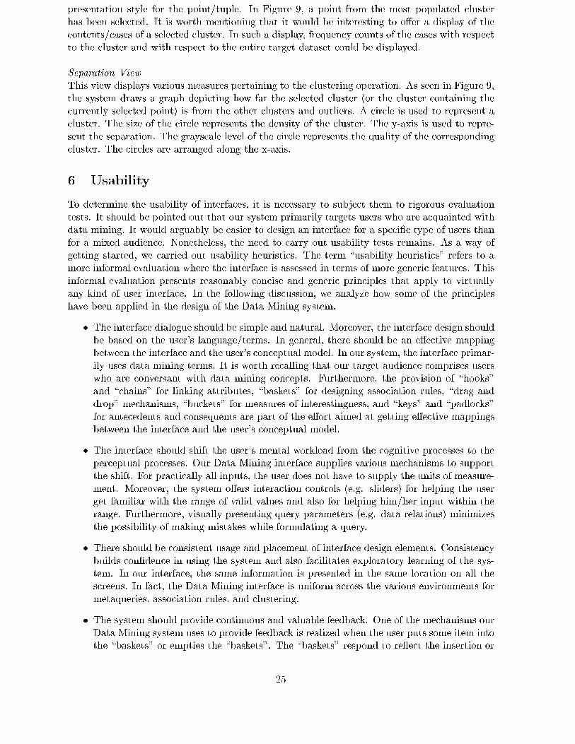
presentation style for the point/tuple. In Figure 9, a point from the most populated cluster

has been selected. It is worth mentioning that it would be interesting to o�er a display of the

contents/cases of a selected cluster. In such a display, frequency counts of the cases with respect

to the cluster and with respect to the entire target dataset could be displayed.

Separation View

This view displays various measures pertaining to the clustering operation. As seen in Figure 9,

the system draws a graph depicting how far the selected cluster (or the cluster containing the

currently selected point) is from the other clusters and outliers. A circle is used to represent a

cluster. The size of the circle represents the density of the cluster. The y-axis is used to repre-

sent the separation. The grayscale level of the circle represents the quality of the corresponding

cluster. The circles are arranged along the x-axis.

6 Usability

To determine the usability of interfaces, it is necessary to subject them to rigorous evaluation

tests. It should be pointed out that our system primarily targets users who are acquainted with

data mining. It would arguably be easier to design an interface for a speci�c type of users than

for a mixed audience. Nonetheless, the need to carry out usability tests remains. As a way of

getting started, we carried out usability heuristics. The term \usability heuristics" refers to a

more informal evaluation where the interface is assessed in terms of more generic features. This

informal evaluation presents reasonably concise and generic principles that apply to virtually

any kind of user interface. In the following discussion, we analyze how some of the principles

have been applied in the design of the Data Mining system.

� The interface dialogue should be simple and natural. Moreover, the interface design should

be based on the user's language/terms. In general, there should be an e�ective mapping

between the interface and the user's conceptual model. In our system, the interface primar-

ily uses data mining terms. It is worth recalling that our target audience comprises users

who are conversant with data mining concepts. Furthermore, the provision of \hooks"

and \chains" for linking attributes, \baskets" for designing association rules, \drag and

drop" mechanisms, \buckets" for measures of interestingness, and \keys" and \padlocks"

for antecedents and consequents are part of the e�ort aimed at getting e�ective mappings

between the interface and the user's conceptual model.

� The interface should shift the user's mental workload from the cognitive processes to the

perceptual processes. Our Data Mining interface supplies various mechanisms to support

the shift. For practically all inputs, the user does not have to supply the units of measure-

ment. Moreover, the system o�ers interaction controls (e.g. sliders) for helping the user

get familiar with the range of valid values and also for helping him/her input within the

range. Furthermore, visually presenting query parameters (e.g. data relations) minimizes

the possibility of making mistakes while formulating a query.

� There should be consistent usage and placement of interface design elements. Consistency

builds con�dence in using the system and also facilitates exploratory learning of the sys-

tem. In our interface, the same information is presented in the same location on all the

screens. In fact, the Data Mining interface is uniform across the various environments for

metaqueries, association rules, and clustering.

� The system should provide continuous and valuable feedback. One of the mechanisms our

Data Mining system uses to provide feedback is realized when the user puts some item into

the \baskets" or empties the \baskets". The \baskets" respond to re ect the insertion or

25

the removal. Moreover, the visualization dynamically updates itself as the user changes

(or interacts with) data mining parameters.

� There is a need to provide shortcuts especially for frequently used operations. In the Data

Mining interface, there are various shortcut mechanisms. For instance double clicking and

single key press commands. The anticipated incorporation of a visual query language is

expected to also help with respect to shortcuts.

� There are many situations that could potentially lead to errors. Adopting an interface

design that prevents error situations from occurring would be of great bene�t. In fact, the

need for error prevention mechanisms arises before (but does not eliminate) the need to

provide valuable error messages. Our Data Mining interface o�ers mechanisms to prevent

invalid inputs (e.g. speci�cation by selection, speci�cation through sliders). It also provides

some status indicators (e.g. when an item is put in a \basket", the status of the \basket"

changes to indicate containment).

Moreover, we carried out some informal user tests on a previous version of the prototype

with data mining experts. We got encouraging results from the tests and even suggestions on

how to improve the interface.

For instance, with respect to clustering, the data mining experts suggested that the system

should provide an optional interaction environment speci�cally designed for the expert user and

still leave the user with the freedom to switch between the two. The optional environment would

allow the user to specify more speci�c clustering parameters (such as choosing an algorithm,

specifying the number of iterations, and putting weights on cases).

7 Future Work

As was suggested by the data mining experts, we are considering the provision of an optional

clustering interaction environment speci�cally designed for the expert user and still leave the

user with the freedom to switch as s/he desires. There is also an intention to include support

for displaying clustering output using a non-Euclidean space. Moreover, as observed earlier, the

incorporation of an optional display for showing the contents of a selected cluster with their

frequency counts is worth consideration.

The current interface and the various data mining visualizations will later be subjected to

formal usability tests. The results obtained from the tests would be instrumental in determining

further relevant interface improvements and modi�cations.

Work aimed at widening the spectrum of data mining strategies supported by the current

system is also going on. Toward providing more user support in the data mining process, plans

are underway to incorporate a visual query language, including its syntax and semantics. At

present, there is a partial prototype of the Data Mining system. The complete implementation

of the same is underway.

26

Part III

Formal Semantics(Paolo Ciaccia, Giovambattista Ianni, Stefano Lodi,

Luigi Palopoli, Marco Patella, Claudio Sartori)

8 Metarules interchange format

The meta-language nature of XML allows to easily de�ne interchange formats and new lan-

guages. Developers are able to design structured, yet easily readable, formats without diÆculty.

Nonetheless, XML data may be exchanged through the Internet allowing the introduction of

many distributed applications (e.g. SOAP based applications [7]).

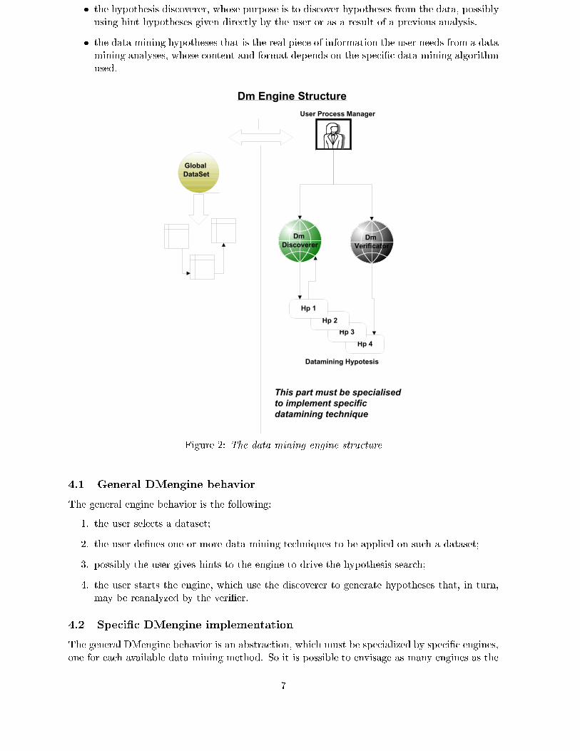
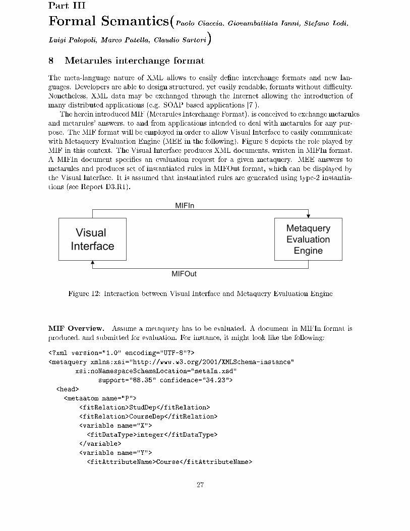
The herein introducedMIF (Metarules Interchange Format), is conceived to exchange metarules

and metarules' answers, to and from applications intended to deal with metarules for any pur-

pose. The MIF format will be employed in order to allow Visual Interface to easily communicate

with Metaquery Evaluation Engine (MEE in the following). Figure 8 depicts the role played by

MIF in this context. The Visual Interface produces XML documents, written in MIFIn format.

A MIFIn document speci�es an evaluation request for a given metaquery. MEE answers to

metarules and produces set of instantiated rules in MIFOut format, which can be displayed by

the Visual Interface. It is assumed that instantiated rules are generated using type-2 instantia-

tions (see Report D3.R1).

Figure 12: Interaction between Visual Interface and Metaquery Evaluation Engine

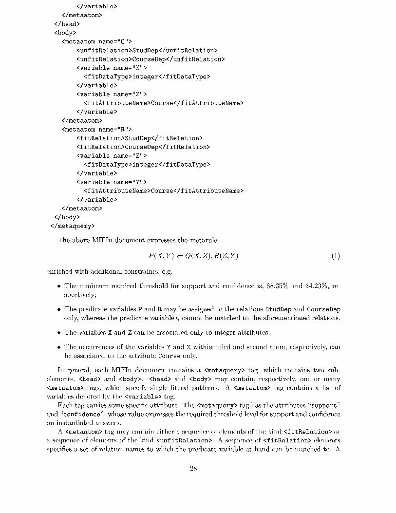
MIF Overview. Assume a metaquery has to be evaluated. A document in MIFIn format is

produced, and submitted for evaluation. For instance, it might look like the following:

<?xml version="1.0" encoding="UTF-8"?>

<metaquery xmlns:xsi="http://www.w3.org/2001/XMLSchema-instance"

xsi:noNamespaceSchemaLocation="metaIn.xsd"

support="88.35" confidence="34.23">

<head>

<metaatom name="P">

<fitRelation>StudDep</fitRelation>

<fitRelation>CourseDep</fitRelation>

<variable name="X">

<fitDataType>integer</fitDataType>

</variable>

<variable name="Y">

<fitAttributeName>Course</fitAttributeName>

27

</variable>

</metaatom>

</head>

<body>

<metaatom name="Q">

<unfitRelation>StudDep</unfitRelation>

<unfitRelation>CourseDep</unfitRelation>

<variable name="X">


</variable>

<variable name="Z">


</variable>

</metaatom>

<metaatom name="R">

<fitRelation>StudDep</fitRelation>

<fitRelation>CourseDep</fitRelation>

<variable name="Z">


</variable>

<variable name="Y">


</variable>

</metaatom>

</body>

</metaquery>

The above MIFIn document expresses the metarule

P (X;Y )( Q(X;Z); R(Z; Y ) (1)

enriched with additional constraints, e.g.

� The minimum required threshold for support and con�dence is, 88.35% and 34.23%, re-

spectively;

� The predicate variables P and R may be assigned to the relations StudDep and CourseDep

only, whereas the predicate variable Q cannot be matched to the aforementioned relations.

� The variables X and Z can be associated only to integer attributes.

� The occurrences of the variables Y and Z within third and second atom, respectively, can

be associated to the attribute Course only.

In general, each MIFIn document contains a <metaquery> tag, which contains two sub-

elements, <head> and <body>. <head> and <body> may contain, respectively, one or many

<metaatom> tags, which specify single literal patterns. A <metaatom> tag contains a list of

variables denoted by the <variable> tag.

Each tag carries some speci�c attribute. The <metaquery> tag has the attributes \support"

and \confidence", whose value expresses the required threshold level for support and con�dence

on instantiated answers.

A <metaatom> tag may contain either a sequence of elements of the kind <fitRelation> or

a sequence of elements of the kind <unfitRelation>. A sequence of <fitRelation> elements

speci�es a set of relation names to which the predicate variable at hand can be matched to. A

28

sequence of <unfitRelation> elements speci�es a set of relation names to which the predicate

variable at hand cannot be matched to, instead. If none of the above sequences are present, a

predicate variable may be freely matched to any relation. A <metaatom> contains anyway a list

of <variable> tags, which speci�es the set of ordinary variables associated to the metaatom at

hand.

The meaning of the elements <fitAttributeName> and <unfitAttributeName> contained within

the <variable> element is symmetric to the elements <fitRelation> and <unfitRelation> of

the <metaatom> tag.

The element <fitDataType> (resp. <unfitDataType>) may be employed in order to specify

which data type the variable at hand could be matched to (resp. not matched to). Note that

it is possible to employ these statement within any occurrence of the tag <variable>, referring

to the variable at hand.

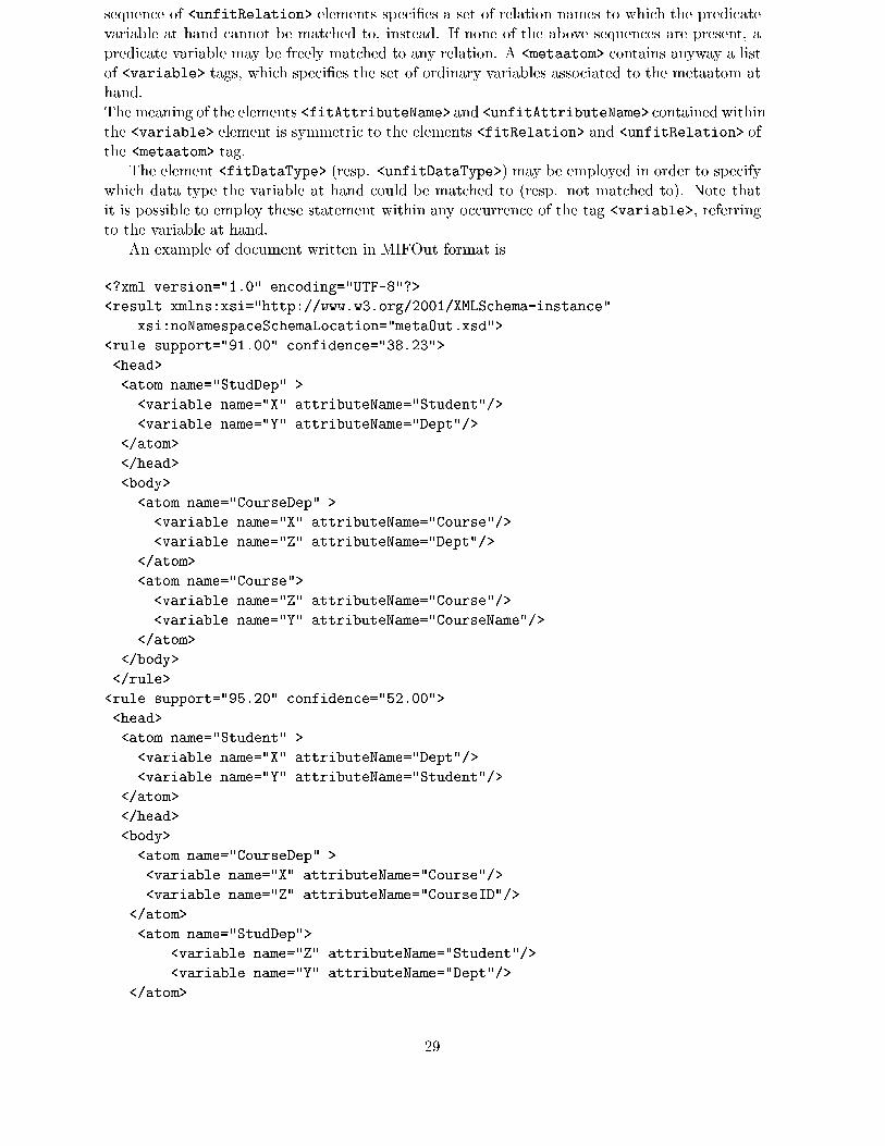
An example of document written in MIFOut format is

<?xml version="1.0" encoding="UTF-8"?>

<result xmlns:xsi="http://www.w3.org/2001/XMLSchema-instance"

xsi:noNamespaceSchemaLocation="metaOut.xsd">

<rule support="91.00" confidence="38.23">

<head>

<atom name="StudDep" >

<variable name="X" attributeName="Student"/>

<variable name="Y" attributeName="Dept"/>

</atom>

</head>

<body>

<atom name="CourseDep" >

<variable name="X" attributeName="Course"/>

<variable name="Z" attributeName="Dept"/>

</atom>

<atom name="Course">

<variable name="Z" attributeName="Course"/>

<variable name="Y" attributeName="CourseName"/>

</atom>

</body>

</rule>

<rule support="95.20" confidence="52.00">

<head>

<atom name="Student" >

<variable name="X" attributeName="Dept"/>

<variable name="Y" attributeName="Student"/>

</atom>

</head>

<body>

<atom name="CourseDep" >

<variable name="X" attributeName="Course"/>

<variable name="Z" attributeName="CourseID"/>

</atom>

<atom name="StudDep">

<variable name="Z" attributeName="Student"/>

<variable name="Y" attributeName="Dept"/>

</atom>

29

</body>

</rule>

</result>

The MIFOut format is simpler than MIFIn, since it is designed to transport sets of instan-

tiated rules giving necessary details on how instantiations were performed. For instance, the

above document encodes the following set of instantiated rules:

studDep(X;Y ) ( courseDep(X;Z); course(Z; Y ): (2)

student(X;Y ) ( courseDep(X;Z); studDep(Z; Y ): (3)

Additional information are provided in order to specify how variables are matched to attributes.

For example, considering rule 2 the occurrence of the variable X within the atom studDep(X;Y )

is bound to the attribute Dept of the studDep table.

In general, a document in MIFOut format contains a sequence of rules. Each rule carries

a list of variables, and for each variable, it is speci�ed which is the bound attribute. A full

speci�cation for the two formats follows.

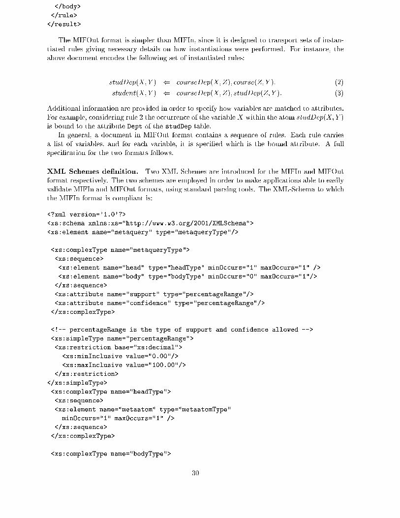
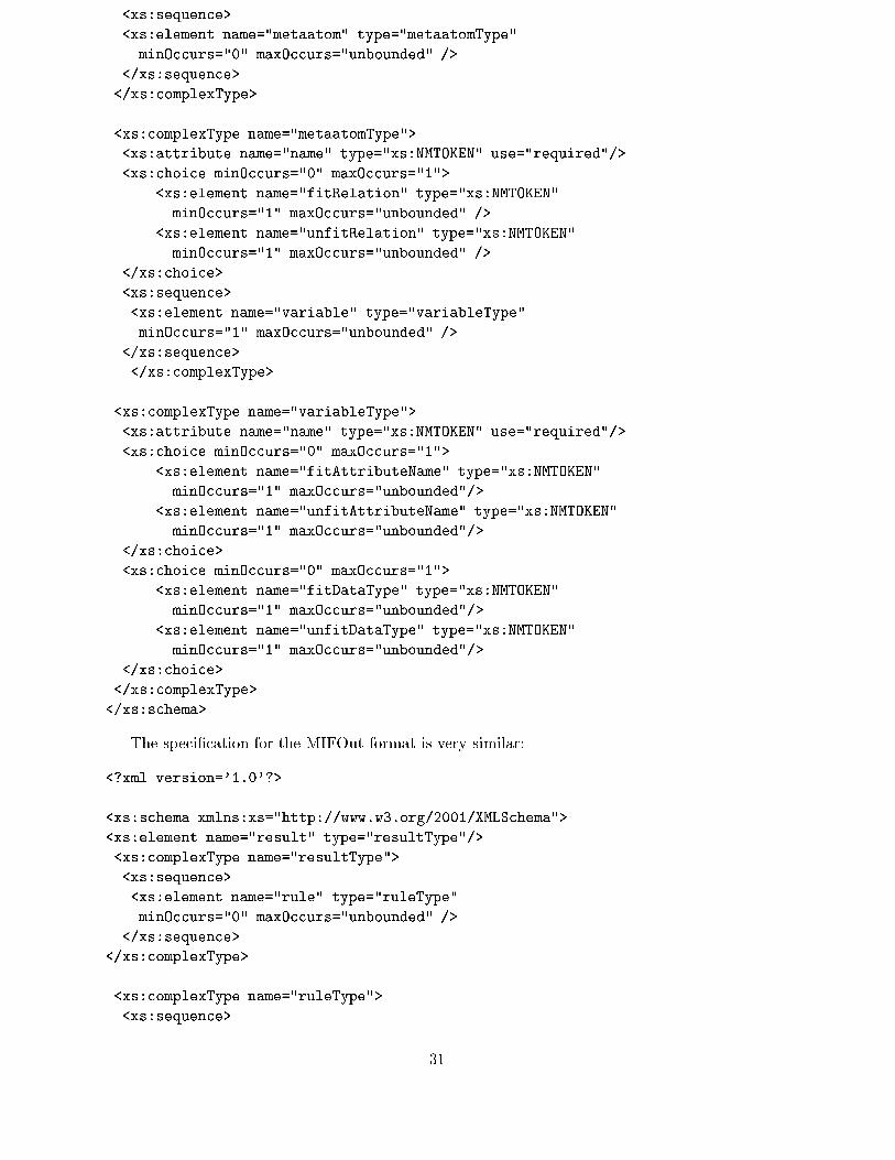
XML Schemes de�nition. Two XML Schemes are introduced for the MIFIn and MIFOut

format respectively. The two schemes are employed in order to make applications able to easily

validate MIFIn and MIFOut formats, using standard parsing tools. The XML-Schema to which

the MIFIn format is compliant is:

<?xml version='1.0'?>

<xs:schema xmlns:xs="http://www.w3.org/2001/XMLSchema">

<xs:element name="metaquery" type="metaqueryType"/>

<xs:complexType name="metaqueryType">

<xs:sequence>

<xs:element name="head" type="headType" minOccurs="1" maxOccurs="1" />

<xs:element name="body" type="bodyType" minOccurs="0" maxOccurs="1"/>

</xs:sequence>

<xs:attribute name="support" type="percentageRange"/>

<xs:attribute name="confidence" type="percentageRange"/>

</xs:complexType>



<xs:simpleType name="percentageRange">

<xs:restriction base="xs:decimal">

<xs:minInclusive value="0.00"/>

<xs:maxInclusive value="100.00"/>

</xs:restriction>

</xs:simpleType>

<xs:complexType name="headType">

<xs:sequence>

<xs:element name="metaatom" type="metaatomType"

minOccurs="1" maxOccurs="1" />

</xs:sequence>

</xs:complexType>

<xs:complexType name="bodyType">

30

<xs:sequence>

<xs:element name="metaatom" type="metaatomType"

minOccurs="0" maxOccurs="unbounded" />

</xs:sequence>

</xs:complexType>

<xs:complexType name="metaatomType">

<xs:attribute name="name" type="xs:NMTOKEN" use="required"/>

<xs:choice minOccurs="0" maxOccurs="1">

<xs:element name="fitRelation" type="xs:NMTOKEN"


<xs:element name="unfitRelation" type="xs:NMTOKEN"


</xs:choice>

<xs:sequence>

<xs:element name="variable" type="variableType"


</xs:sequence>

</xs:complexType>

<xs:complexType name="variableType">



<xs:element name="fitAttributeName" type="xs:NMTOKEN"

minOccurs="1" maxOccurs="unbounded"/>

<xs:element name="unfitAttributeName" type="xs:NMTOKEN"


</xs:choice>


<xs:element name="fitDataType" type="xs:NMTOKEN"


<xs:element name="unfitDataType" type="xs:NMTOKEN"


</xs:choice>

</xs:complexType>

</xs:schema>

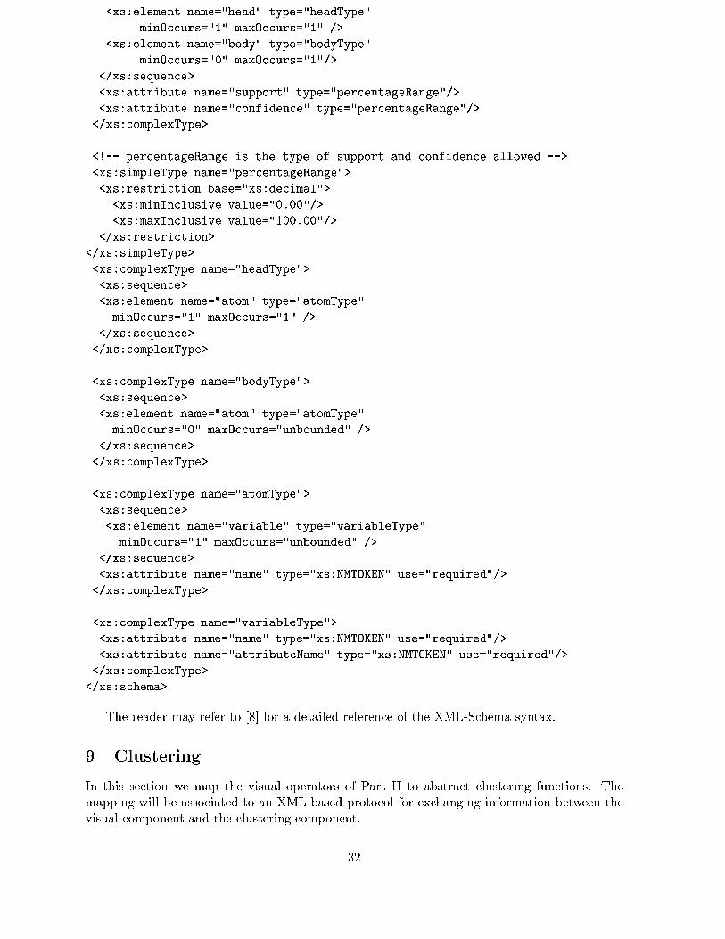
The speci�cation for the MIFOut format is very similar:

<?xml version='1.0'?>

<xs:schema xmlns:xs="http://www.w3.org/2001/XMLSchema">

<xs:element name="result" type="resultType"/>

<xs:complexType name="resultType">

<xs:sequence>

<xs:element name="rule" type="ruleType"


</xs:sequence>

</xs:complexType>

<xs:complexType name="ruleType">

<xs:sequence>

31

<xs:element name="head" type="headType"


<xs:element name="body" type="bodyType"

minOccurs="0" maxOccurs="1"/>

</xs:sequence>

<xs:attribute name="support" type="percentageRange"/>

<xs:attribute name="confidence" type="percentageRange"/>

</xs:complexType>



<xs:simpleType name="percentageRange">

<xs:restriction base="xs:decimal">

<xs:minInclusive value="0.00"/>

<xs:maxInclusive value="100.00"/>

</xs:restriction>

</xs:simpleType>

<xs:complexType name="headType">

<xs:sequence>

<xs:element name="atom" type="atomType"


</xs:sequence>

</xs:complexType>

<xs:complexType name="bodyType">

<xs:sequence>

<xs:element name="atom" type="atomType"


</xs:sequence>

</xs:complexType>

<xs:complexType name="atomType">

<xs:sequence>

<xs:element name="variable" type="variableType"


</xs:sequence>


</xs:complexType>

<xs:complexType name="variableType">


<xs:attribute name="attributeName" type="xs:NMTOKEN" use="required"/>

</xs:complexType>

</xs:schema>

The reader may refer to [8] for a detailed reference of the XML-Schema syntax.

9 Clustering

In this section we map the visual operators of Part II to abstract clustering functions. The

mapping will be associated to an XML-based protocol for exchanging information between the

visual component and the clustering component.

32

The Data Mining Group has recently developed a industrial XML-based standard for the

exchange of results between mining applications, named Predictive Model Markup Language.

The standard is published as a XML DTD speci�cation allowing for the description of a variety

of data models, including descriptive statistics, trees, regression, and clustering. Although the

speci�cation is almost entirely satisfactory w.r.t. the description of the result of a mining task,

no provision is made for the description of the input to a mining task, which is by nature

algorithm-dependent.

In Section 9.1 we de�ne a XML DTD for the speci�cation of parameters and other information

as input by the clustering component. In Section 9.2 we evaluate PMML 2.0 and describe an

update which allows for the representation of the results of a clustering task.

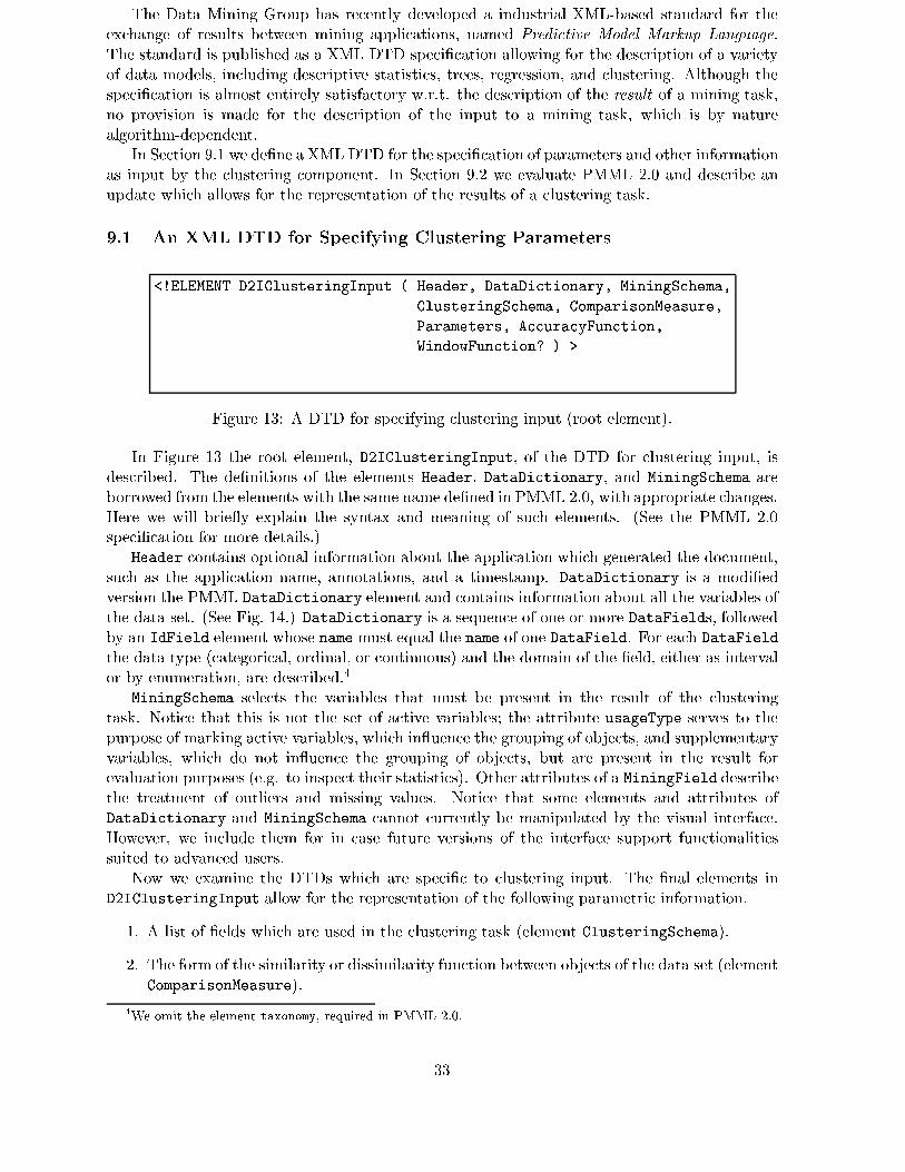
9.1 An XML DTD for Specifying Clustering Parameters

<!ELEMENT D2IClusteringInput ( Header, DataDictionary, MiningSchema,

ClusteringSchema, ComparisonMeasure,

Parameters, AccuracyFunction,

WindowFunction? ) >

Figure 13: A DTD for specifying clustering input (root element).

In Figure 13 the root element, D2IClusteringInput, of the DTD for clustering input, is

described. The de�nitions of the elements Header, DataDictionary, and MiningSchema are

borrowed from the elements with the same name de�ned in PMML 2.0, with appropriate changes.

Here we will brie y explain the syntax and meaning of such elements. (See the PMML 2.0

speci�cation for more details.)

Header contains optional information about the application which generated the document,

such as the application name, annotations, and a timestamp. DataDictionary is a modi�ed

version the PMML DataDictionary element and contains information about all the variables of

the data set. (See Fig. 14.) DataDictionary is a sequence of one or more DataFields, followed

by an IdField element whose name must equal the name of one DataField. For each DataField

the data type (categorical, ordinal, or continuous) and the domain of the �eld, either as interval

or by enumeration, are described.4

MiningSchema selects the variables that must be present in the result of the clustering

task. Notice that this is not the set of active variables; the attribute usageType serves to the

purpose of marking active variables, which in uence the grouping of objects, and supplementary

variables, which do not in uence the grouping of objects, but are present in the result for

evaluation purposes (e.g. to inspect their statistics). Other attributes of a MiningField describe

the treatment of outliers and missing values. Notice that some elements and attributes of

DataDictionary and MiningSchema cannot currently be manipulated by the visual interface.

However, we include them for in case future versions of the interface support functionalities

suited to advanced users.

Now we examine the DTDs which are speci�c to clustering input. The �nal elements in

D2IClusteringInput allow for the representation of the following parametric information.

1. A list of �elds which are used in the clustering task (element ClusteringSchema).

2. The form of the similarity or dissimilarity function between objects of the data set (element

ComparisonMeasure).

4We omit the element taxonomy, required in PMML 2.0.

33

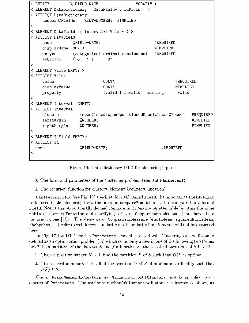
<!ENTITY % FIELD-NAME "CDATA" >

<!ELEMENT DataDictionary ( DataField+ , IdField ) >

<!ATTLIST DataDictionary

numberOfFields %INT-NUMBER; #IMPLIED

>

<!ELEMENT DataField ( Interval*| Value* ) >

<!ATTLIST DataField

name %FIELD-NAME; #REQUIRED

displayName CDATA #IMPLIED

optype (categorical|ordinal|continuous) #REQUIRED

isCyclic ( 0 | 1 ) "0"

>

<!ELEMENT Value EMPTY >

<!ATTLIST Value

value CDATA #REQUIRED

displayValue CDATA #IMPLIED

property (valid | invalid | missing) "valid"

>

<!ELEMENT Interval EMPTY>

<!ATTLIST Interval

closure (openClosed|openOpen|closedOpen|closedClosed) #REQUIRED

leftMargin %NUMBER; #IMPLIED

rightMargin %NUMBER; #IMPLIED

>

<!ELEMENT IdField EMPTY>

<!ATTLIST Id


>

Figure 14: Data dictionary DTD for clustering input.

3. The form and parameters of the clustering problem (element Parameters).

4. The accuracy function for clusters (element AccuracyFunction).

ClusteringField (see Fig. 16) speci�es, for �eld named field, the importance fieldWeight

to be used in the clustering task, the function compareFunction used to compare the values of

field. Notice that extensionally de�ned compare functions are representable by using the value

table of compareFunction and specifying a list of Comparisons elements (not shown here

for brevity, see [13]). The elements of ComparisonMeasure (euclidean, squaredEuclidean,

chebychev,. . . ) refer to well-known similarity or dissimilarity functions and will not be discussed

here.

In Fig. 17 the DTD for the Parameters element is described. Clustering can be formally

de�ned as an optimization problem [14] which commonly arises in one of the following two forms.

Let P be a partition of the data set S and f a function on the set of all partitions of S into R+ .

1. Given a positive integer K > 1, �nd the partition P of S such that f(P) is optimal.

2. Given a real number � 2 R+ , �nd the partition P of S of minimum cardinality such that

f(P) � �.

One of FixedNumberOfClusters and MinimumNumberOfClusters must be speci�ed as el-

ements of Parameters. The attribute numberOfClusters will store the integer K above, as

34

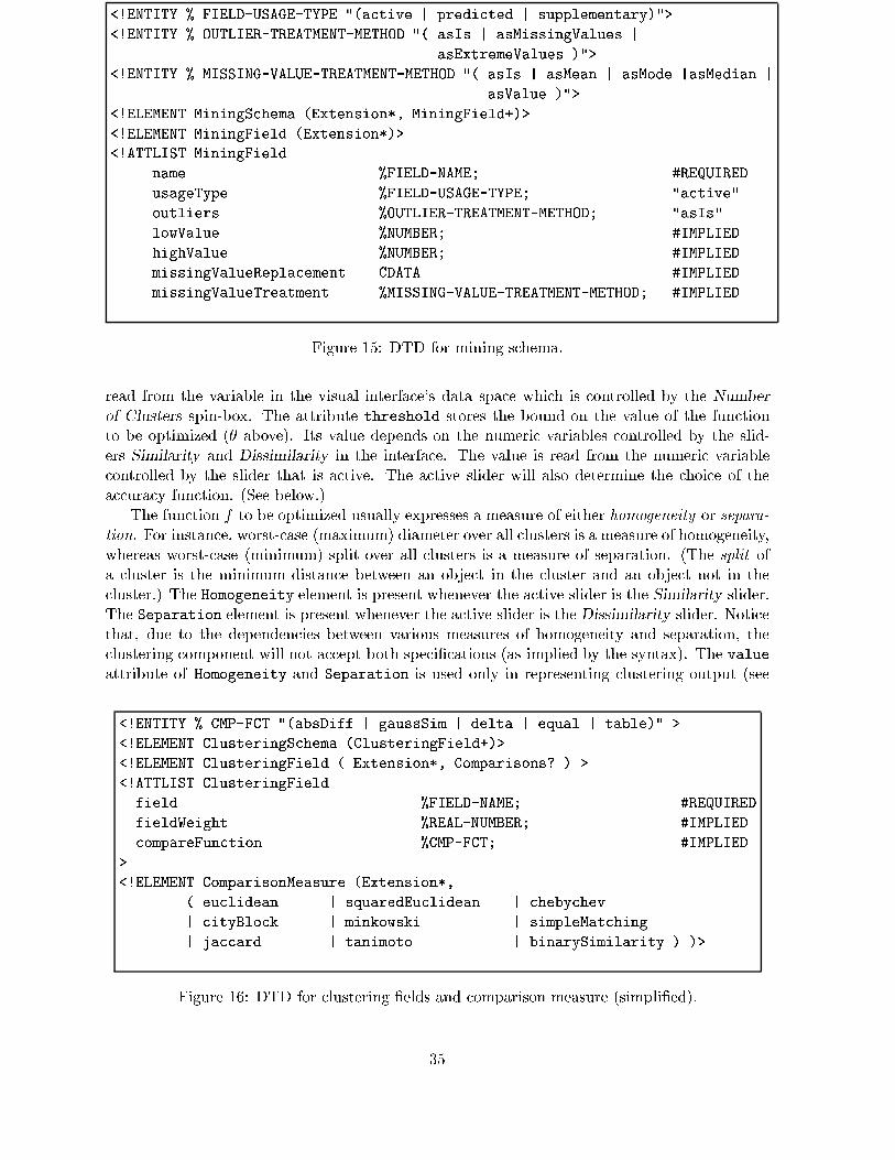
<!ENTITY % FIELD-USAGE-TYPE "(active | predicted | supplementary)">

<!ENTITY % OUTLIER-TREATMENT-METHOD "( asIs | asMissingValues |

asExtremeValues )">

<!ENTITY % MISSING-VALUE-TREATMENT-METHOD "( asIs | asMean | asMode |asMedian |

asValue )">

<!ELEMENT MiningSchema (Extension*, MiningField+)>

<!ELEMENT MiningField (Extension*)>

<!ATTLIST MiningField


usageType %FIELD-USAGE-TYPE; "active"

outliers %OUTLIER-TREATMENT-METHOD; "asIs"

lowValue %NUMBER; #IMPLIED

highValue %NUMBER; #IMPLIED

missingValueReplacement CDATA #IMPLIED

missingValueTreatment %MISSING-VALUE-TREATMENT-METHOD; #IMPLIED

Figure 15: DTD for mining schema.

read from the variable in the visual interface's data space which is controlled by the Number

of Clusters spin-box. The attribute threshold stores the bound on the value of the function

to be optimized (� above). Its value depends on the numeric variables controlled by the slid-

ers Similarity and Dissimilarity in the interface. The value is read from the numeric variable

controlled by the slider that is active. The active slider will also determine the choice of the

accuracy function. (See below.)

The function f to be optimized usually expresses a measure of either homogeneity or separa-

tion. For instance, worst-case (maximum) diameter over all clusters is a measure of homogeneity,

whereas worst-case (minimum) split over all clusters is a measure of separation. (The split of

a cluster is the minimum distance between an object in the cluster and an object not in the

cluster.) The Homogeneity element is present whenever the active slider is the Similarity slider.

The Separation element is present whenever the active slider is the Dissimilarity slider. Notice

that, due to the dependencies between various measures of homogeneity and separation, the

clustering component will not accept both speci�cations (as implied by the syntax). The value

attribute of Homogeneity and Separation is used only in representing clustering output (see

<!ENTITY % CMP-FCT "(absDiff | gaussSim | delta | equal | table)" >

<!ELEMENT ClusteringSchema (ClusteringField+)>

<!ELEMENT ClusteringField ( Extension*, Comparisons? ) >

<!ATTLIST ClusteringField

field %FIELD-NAME; #REQUIRED

fieldWeight %REAL-NUMBER; #IMPLIED

compareFunction %CMP-FCT; #IMPLIED

>

<!ELEMENT ComparisonMeasure (Extension*,

( euclidean | squaredEuclidean | chebychev

| cityBlock | minkowski | simpleMatching

| jaccard | tanimoto | binarySimilarity ) )>

Figure 16: DTD for clustering �elds and comparison measure (simpli�ed).

35

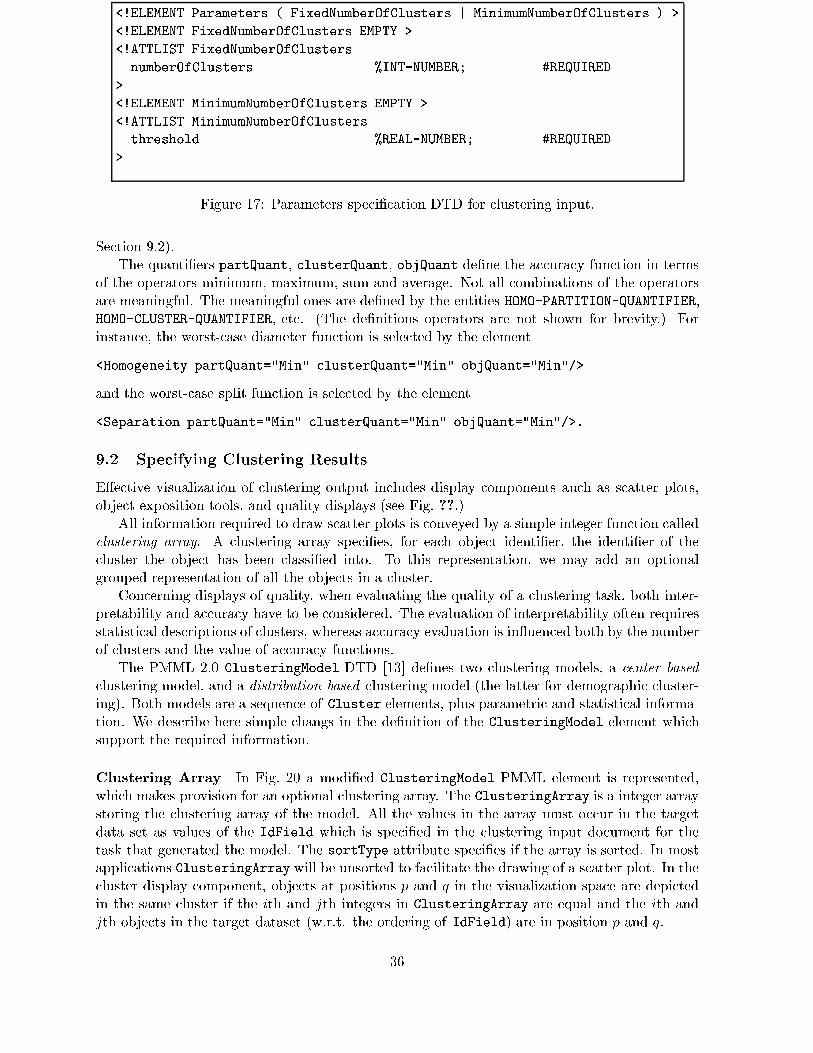
<!ELEMENT Parameters ( FixedNumberOfClusters | MinimumNumberOfClusters ) >

<!ELEMENT FixedNumberOfClusters EMPTY >

<!ATTLIST FixedNumberOfClusters

numberOfClusters %INT-NUMBER; #REQUIRED

>

<!ELEMENT MinimumNumberOfClusters EMPTY >

<!ATTLIST MinimumNumberOfClusters

threshold %REAL-NUMBER; #REQUIRED

>

Figure 17: Parameters speci�cation DTD for clustering input.

Section 9.2).

The quanti�ers partQuant, clusterQuant, objQuant de�ne the accuracy function in terms

of the operators minimum, maximum, sum and average. Not all combinations of the operators

are meaningful. The meaningful ones are de�ned by the entities HOMO-PARTITION-QUANTIFIER,

HOMO-CLUSTER-QUANTIFIER, etc. (The de�nitions operators are not shown for brevity.) For

instance, the worst-case diameter function is selected by the element

<Homogeneity partQuant="Min" clusterQuant="Min" objQuant="Min"/>

and the worst-case split function is selected by the element

<Separation partQuant="Min" clusterQuant="Min" objQuant="Min"/>.

9.2 Specifying Clustering Results

E�ective visualization of clustering output includes display components auch as scatter plots,

object exposition tools, and quality displays (see Fig. ??.)

All information required to draw scatter plots is conveyed by a simple integer function called

clustering array. A clustering array speci�es, for each object identi�er, the identi�er of the

cluster the object has been classi�ed into. To this representation, we may add an optional

grouped representation of all the objects in a cluster.

Concerning displays of quality, when evaluating the quality of a clustering task, both inter-

pretability and accuracy have to be considered. The evaluation of interpretability often requires

statistical descriptions of clusters, whereas accuracy evaluation is in uenced both by the number

of clusters and the value of accuracy functions.

The PMML 2.0 ClusteringModel DTD [13] de�nes two clustering models, a center based

clustering model, and a distribution based clustering model (the latter for demographic cluster-

ing). Both models are a sequence of Cluster elements, plus parametric and statistical informa-

tion. We describe here simple changs in the de�nition of the ClusteringModel element which

support the required information.

Clustering Array In Fig. 20 a modi�ed ClusteringModel PMML element is represented,

which makes provision for an optional clustering array. The ClusteringArray is a integer array

storing the clustering array of the model. All the values in the array must occur in the target

data set as values of the IdField which is speci�ed in the clustering input document for the

task that generated the model. The sortType attribute speci�es if the array is sorted. In most

applications ClusteringArray will be unsorted to facilitate the drawing of a scatter plot. In the

cluster display component, objects at positions �p and �q in the visualization space are depicted

in the same cluster if the ith and jth integers in ClusteringArray are equal and the ith and

jth objects in the target dataset (w.r.t. the ordering of IdField) are in position �p and �q.

36

Descriptive Statistics Although statistical descriptions are currently not supported by the

system, they are already present in PMML. Both in center-based and distribution-based models,

the speci�cation allows for utilizing a large number of descriptive statistics. For any mining �eld,

background/per cluster discrete and continuous statistics can be represented, including mean,

standard deviation, quantiles, and case frequencies. As a result, the speci�cation supports the

comparison of relative frequency counts with respect to a cluster and the entire target data set

in the visual interface, e.g. by overlapping pie charts or histograms.

Accuracy Feedback The speci�cation of the Cluster element does not include explicit sup-

port of accuracy functions. Consequently, the PMML standard has to be extended to support

homogeneity or separation measures. (The computation of these functions in the visual interface

would be ineÆcient.) To this purpose we introduce a new optional element AccuracyFeedback

in the Cluster DTD of the PMML speci�cation (see Fig. 21). Notice that it is legal to list

an arbitrary number of accuracy functions. This can be helpful in situations where the user is

searching for a compromise between di�erent measures of accuracy. The system currently sup-

ports only a separation function per clustering task. Therefore, the content of the visual interface

variable storing the position on the Separation axis of cluster named name in the Separation

View has to be set according to the value attribute of the �rst AccuracyFeedback|Separation

of the Cluster having name=name.

9.3 Example

In Part II a simple example of a data set for the clustering task is presented. Here we extend the

example, specifying an XML �le for clustering input, which conforms to the D2IClusteringInput

DTD, and an XML �le for clustering output, which conforms to the modi�ed PMMLDTD, whose

root element we name D2IClusteringOutput.

In the input document (see Fig. 22), the active variables are the towns' coordinates TwX

and TwY. The supplementary variable TwYEst will not in uence clustering, but will be in the

output document. In ClusteringSchema, we select absolute di�erence as the function to com-

pare values of each variable. ComparisonMeasure selects Euclidean distance. Parameters and

AccuracyFunction select a separation function de�ned as the worst-case case split over the

clusters in the partition.

The output document (see Fig. 23) is the result of appliyng the well-known single link

hierarchical algorithm to the data set, halting at the topmost partition whose single link value

is less than three. (It is well known that the single link algorithm �nds the optimum solution

for the worst-case split function at any level of the hierarchy [14].) For brevity, we omit the

background statistics ModelStats and all information which is copied unchanged from the input

document. The model describes four clusters named from 1 to 4 in the Cluster elements. Each

cluster contains its split value and the maximum distance between its objects, i.e. the cluster's

diameter. Finally, a clustering array assigns each object to its cluster: objects that are �rst and

second in TwId to cluster named 1, third, fourth and �fth to 2, sixth and seventh to 3, and the

eigth object to the singleton cluster 4.

10 Approximate Similarity Queries

The current trend in data mining is to make the data mining process much more interactive. In

this light, approximate evaluation of similarity queries can dramatically reduce the time required

by the data mining algorithm to produce its results. Quoting from [4]:

The current process is to select parameters, to run a data mining algorithm and,

�nally, to visualize the result of the algorithm. (The) dramatic performance gains

37

could open the potential to make this process so fast that a user may change pa-

rameters and immediately see the resulting changes in the visualization. Here, it

could be bene�cial to apply new concepts in database systems which evaluate queries

approximately or produce �rst results in an early stage of processing.

In the following, we will specify how the system is able to support the formulation of approx-

imate similarity queries, whereas, for the visualization of results, the (Overview + Detail) view

used for clustering can be adopted. In order to specify the semantics of the visual interface, we

adopt the syntax of XUL (XML-based User-interface Language) [24]


In [6, Part III], PAC queries are proposed as a search paradigm for quality-controlled approx-

imate similarity search. In particular, PAC (range and k-NN) queries allow the error on the

query result to exceed a certain threshold (indicated by an accuracy parameter �) with a proba-

bility not higher than the value of the reliability parameter Æ. In order to perform a PAC query,

the user has therefore to specify a value for the accuracy and the reliability parameters � and

Æ. The environment provides two sliders to adjust the values of both accuracy and reliability

parameters from a maximum of 100% (exact query) to a minimum application-speci�c value

(e.g. 50% for both parameters).

Each similarity query requires a reference point to be expressed. The choice of a reference

point can be performed by using two di�erent modalities:

1. By manually entering the coordinates of the point.

2. By clicking on a point within a window.

For the former input modality, the system presents a text box where the user can type the

coordinates of the point he/she is interested in. As for the latter way of specifying the query

point, we rely on the visualization of results from previous data mining tasks. In particular, since

results of clustering are more likely to be used than those of meta-querying or association rules,

we suppose that the user can select the reference point by clicking on it within the \Clusters"

component of the Clustering Output environment (see previous Section).

Finally, the last parameter requested by a PAC query is dependent on the query type. In

particular, for k-NN queries the user has to specify the number k of requested result, whereas

for range queries he/she has to �x the distance threshold that points in the result should not

exceed. The component provides a spin-box for each value, with an alternate input/text-box

where the user can type the requested value. Two radio buttons allow the user to specify the

type of query he/she is interested in, and to activate the corresponding input box, the other

being grayed out. In case that the reference point is graphically chosen by the user by clicking on

a point in the Clustering Output environment, the range query threshold can also be speci�ed

by dragging within the window to specify the query radius: In this modality, a circle is drawn

on the scatter plot, and the value within the input box is changed accordingly, until the user

releases the mouse button. Finally, the torch icon is used to specify to the underlying system to

actually perform the PAC query on the target dataset based on the speci�ed parameters.

De�nition of the Interface using XUL

In the following we provide a simple de�nition of the interface using XUL [24]. It is supposed

that the underlying system supplies two methods, namely PAC kNN and PAC range: In particular:

� PAC kNN takes as input a reference point, an integer value k representing the required result

cardinality, and the values of the accuracy and reliability parameters � and Æ, and returns

a vector of k points.

38

� PAC range takes as input a reference point, a distance value r representing query radius,

and the values of the accuracy and reliability parameters � and Æ, and returns a set of

points.

In the following, we suppose that the corresponding XBL (eXtensible Bindings Language) �le

chrome://PAC/content/PAC.xbl is available, containing the code to communicate with the

PAC kNN and PAC range methods. Note that, in this speci�cation, the component defaults to

range queries.

The next �gure shows the content of the chrome://PAC/content/PAC.xbl �le: Three basic

event handler are provided:

kNN This code is executed whenever the user selects the k best matches radio button, and

activates the correspondent n. of results input box, while graying out the threshold value

input box.

range This code is executed whenever the user selects the max distance radio button, and

activates the correspondent threshold value input box, while graying out the n. of results

input box.

go This code is used to communicate with the underlying system, invoking the PAC kNN and

PAC range methods (that we suppose to be included in the �le) with appropriate values

for each parameter.

References

[1] R. Agrawal and R. Srikant. Fast algorithms for mining association rules. In Twentieth

International Conference on Very Large Data Bases, 1994.

[2] Baeza-Yates and Ribiero-Neto. Modern Information Retrieval. Addison Wesley, 1999.

[3] R. Ben-Eliyahu-Zohary and E. Gudes. Towards eÆcient metaquerying. In Proceedings of

International Joint Conference on Arti�cial Intelligence, 1999.

[4] C. B�ohm. Database systems supporting next decade's applications. Submitted for publica-

tion, 2002.

[5] S. K. Card, J. D. Mackinlay, and B. Shneiderman, editors. Readings in Information

Visualization-Using Vision to Think. Morgan Kaufmann Publishers, 1999.

[6] P. Ciaccia, G. Ianni, S. Lodi, L. Palopoli, M. Patella, and C. Sartori. Methods for cluster-

ing, meta-querying, approximate and similarity search. Technical report, Technical Report

D3.R3 of D2I, Integration, Warehousing, and Mining of Heterogeneous Data Sources, Italian

MIUR Project, http://www.dis.uniroma1.it/~lembo/D2I/, 2001.

[7] W3C Consortium. Soap version 1.2 working draft,

http://www.w3.org/tr/2001/wd-soap12-20010709.

[8] W3C Consortium. Xml schema web site, http://www.w3.org/xml/schema.

[9] C. Domshlak, D. Gershkovich, E. Gudes, N. Liusternik, A. Meisels, T. Rosen, and S. E.

Shimony. Fleximine : A exible platform for kdd research and application construction.

Technical report, BenGurion University, Technical Report FC9804, 1998.

[10] J. F. Elder IV and D. W. Abbott. A comparison of leading data mining tools. In Fourth

International Conference on Knowledge Discovery and Data Mining, 1998.

39

[11] U. Fayyad, G. G. Grinstein, and A. Wierse, editors. Information Visualization in Data

Mining and Knowledge Discovery. Morgan Kaufmann Publishers, 2002.

[12] U. Fayyad, G. Piatetsky-Shapiro, and P. Smyth. Knowledge discovery and data mining-

towards a unifying framework. In Second International Conference on Knowledge Discovery

and Data Mining, 1996.

[13] The Data Mining Group. PMML 2.0 - Predictive Model Markup Language.

http://www.dmg.org/pmmlspecs_v2/pmml_v2_0.html.

[14] Pierre Hansen and Brigitte Jaumard. Cluster analysis and mathematical programming.

Mathematical Programming, 79:191{215, 1997.

[15] IBM. Quest, http://www.almaden.ibm.com/cs/quest.

[16] L. Kaufman and P. J. Rousseeuw. Finding Groups in Data-Introduction to Cluster Analysis.

John Wiley & Sons, 1990.

[17] B. Leing and W. Shen. A metapattern-based automated discovery loop for integrated data

mining-unsupervised learning of relational patterns. In IEEE Transactions on Knowledge

and Data Engineering, 1996.

[18] SGI. Sgi, http://www.sgi.com.

[19] B. Shneiderman. Designing the User Interface-Strategies for E�ective Human-Computer

Interaction. Addison Wesley, 1997.

[20] Accrue Software. Accrue software, inc., http://www.accrue.com.

[21] JDA Software. Jda software group, inc.,http://www.jda.com.

[22] SPSS. Clementine, http://www.spss.com/clementine.

[23] P. C. Wong, P. Whitney, and J. Thomas. Visualizing association rules for text mining. In

Proceedings IEEE Information Visualization, 1999.

[24] XulPlanet. Xul, http://www.xulplanet.com.

40

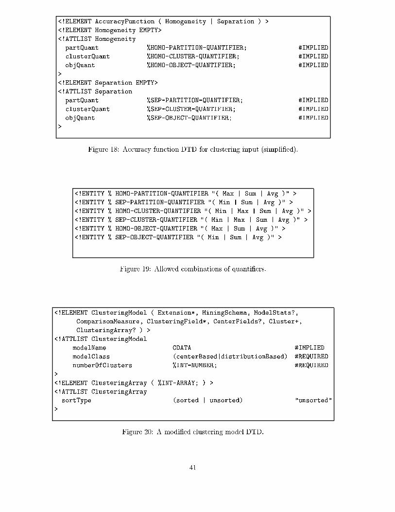
<!ELEMENT AccuracyFunction ( Homogeneity | Separation ) >

<!ELEMENT Homogeneity EMPTY>

<!ATTLIST Homogeneity

partQuant %HOMO-PARTITION-QUANTIFIER; #IMPLIED

clusterQuant %HOMO-CLUSTER-QUANTIFIER; #IMPLIED

objQuant %HOMO-OBJECT-QUANTIFIER; #IMPLIED

>

<!ELEMENT Separation EMPTY>

<!ATTLIST Separation

partQuant %SEP-PARTITION-QUANTIFIER; #IMPLIED

clusterQuant %SEP-CLUSTER-QUANTIFIER; #IMPLIED

objQuant %SEP-OBJECT-QUANTIFIER; #IMPLIED

>

Figure 18: Accuracy function DTD for clustering input (simpli�ed).

<!ENTITY % HOMO-PARTITION-QUANTIFIER "( Max | Sum | Avg )" >

<!ENTITY % SEP-PARTITION-QUANTIFIER "( Min | Sum | Avg )" >

<!ENTITY % HOMO-CLUSTER-QUANTIFIER "( Min | Max | Sum | Avg )" >

<!ENTITY % SEP-CLUSTER-QUANTIFIER "( Min | Max | Sum | Avg )" >

<!ENTITY % HOMO-OBJECT-QUANTIFIER "( Max | Sum | Avg )" >

<!ENTITY % SEP-OBJECT-QUANTIFIER "( Min | Sum | Avg )" >

Figure 19: Allowed combinations of quanti�ers.

<!ELEMENT ClusteringModel ( Extension*, MiningSchema, ModelStats?,

ComparisonMeasure, ClusteringField*, CenterFields?, Cluster+,

ClusteringArray? ) >

<!ATTLIST ClusteringModel

modelName CDATA #IMPLIED

modelClass (centerBased|distributionBased) #REQUIRED

numberOfClusters %INT-NUMBER; #REQUIRED

>

<!ELEMENT ClusteringArray ( %INT-ARRAY; ) >

<!ATTLIST ClusteringArray

sortType (sorted | unsorted) "unsorted"

>

Figure 20: A modi�ed clustering model DTD.

41

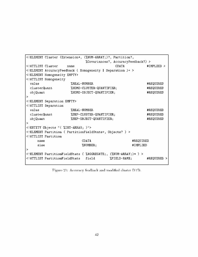
<!ELEMENT Cluster (Extension*, (%NUM-ARRAY;)?, Partition?,

%Covariances?, AccuracyFeedback?) >

<!ATTLIST Cluster name CDATA #IMPLIED >

<!ELEMENT AccuracyFeedback ( Homogeneity | Separation )+ >

<!ELEMENT Homogeneity EMPTY>

<!ATTLIST Homogeneity

value %REAL-NUMBER #REQUIRED

clusterQuant %HOMO-CLUSTER-QUANTIFIER; #REQUIRED

objQuant %HOMO-OBJECT-QUANTIFIER; #REQUIRED

>

<!ELEMENT Separation EMPTY>

<!ATTLIST Separation

value %REAL-NUMBER #REQUIRED

clusterQuant %SEP-CLUSTER-QUANTIFIER; #REQUIRED

objQuant %SEP-OBJECT-QUANTIFIER; #REQUIRED

>

<!ENTITY Objects "( %INT-ARRAY; )">

<!ELEMENT Partition ( PartitionFieldStats+, Objects? ) >

<!ATTLIST Partition

name CDATA #REQUIRED

size %NUMBER; #IMPLIED

>

<!ELEMENT PartitionFieldStats ( %AGGREGATE;, (%NUM-ARRAY;)* ) >

<!ATTLIST PartitionFieldStats field %FIELD-NAME; #REQUIRED >

Figure 21: Accuracy feedback and modi�ed cluster DTD.

42

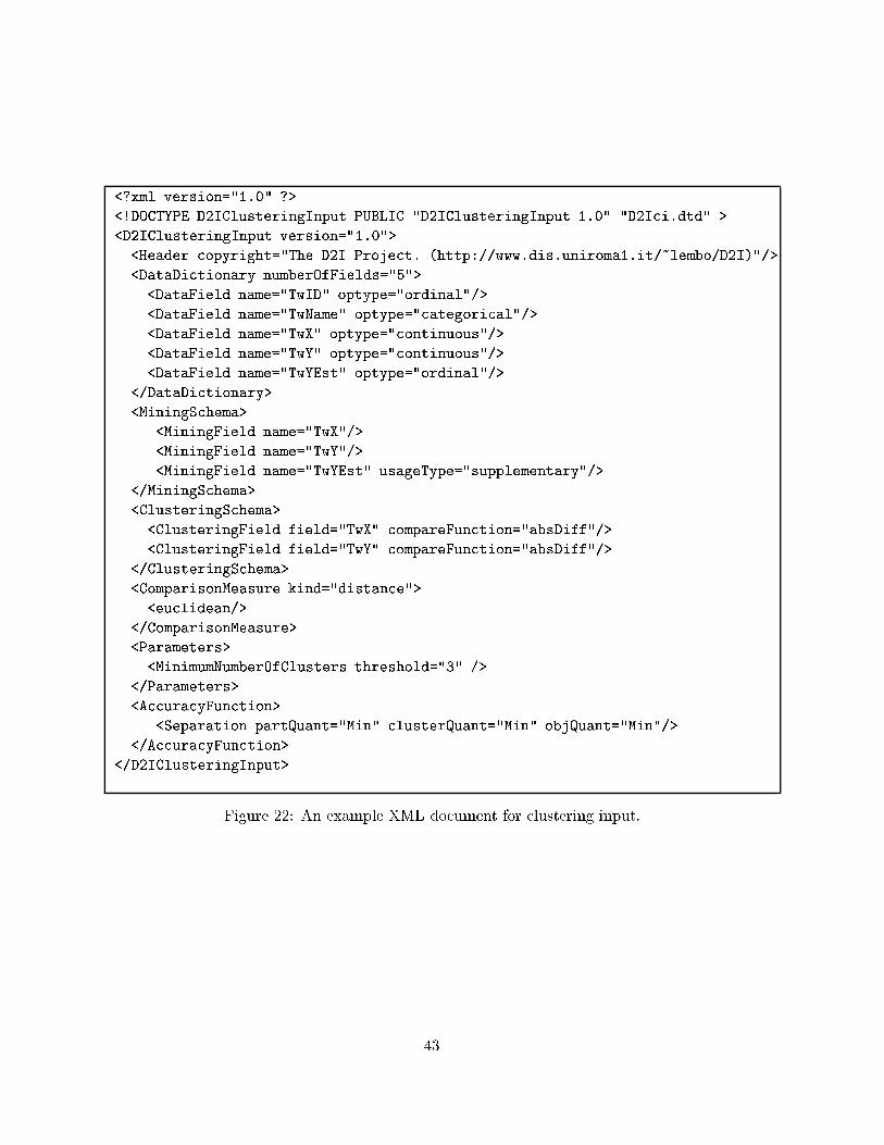
<?xml version="1.0" ?>

<!DOCTYPE D2IClusteringInput PUBLIC "D2IClusteringInput 1.0" "D2Ici.dtd" >

<D2IClusteringInput version="1.0">

<Header copyright="The D2I Project. (http://www.dis.uniroma1.it/~lembo/D2I)"/>

<DataDictionary numberOfFields="5">

<DataField name="TwID" optype="ordinal"/>

<DataField name="TwName" optype="categorical"/>

<DataField name="TwX" optype="continuous"/>

<DataField name="TwY" optype="continuous"/>

<DataField name="TwYEst" optype="ordinal"/>

</DataDictionary>

<MiningSchema>

<MiningField name="TwX"/>

<MiningField name="TwY"/>

<MiningField name="TwYEst" usageType="supplementary"/>

</MiningSchema>

<ClusteringSchema>

<ClusteringField field="TwX" compareFunction="absDiff"/>

<ClusteringField field="TwY" compareFunction="absDiff"/>

</ClusteringSchema>

<ComparisonMeasure kind="distance">

<euclidean/>

</ComparisonMeasure>

<Parameters>

<MinimumNumberOfClusters threshold="3" />

</Parameters>

<AccuracyFunction>

<Separation partQuant="Min" clusterQuant="Min" objQuant="Min"/>

</AccuracyFunction>

</D2IClusteringInput>

Figure 22: An example XML document for clustering input.

43

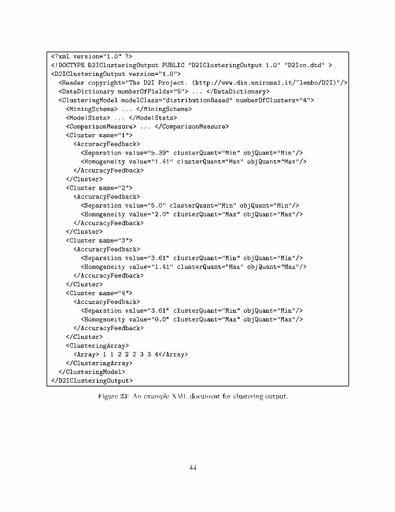
<?xml version="1.0" ?>

<!DOCTYPE D2IClusteringOutput PUBLIC "D2IClusteringOutput 1.0" "D2Ico.dtd" >

<D2IClusteringOutput version="1.0">

<Header copyright="The D2I Project. (http://www.dis.uniroma1.it/~lembo/D2I)"/>

<DataDictionary numberOfFields="5"> ... </DataDictionary>

<ClusteringModel modelClass="distributionBased" numberOfClusters="4">

<MiningSchema> ... </MiningSchema>

<ModelStats> ... </ModelStats>

<ComparisonMeasure> ... </ComparisonMeasure>

<Cluster name="1">

<AccuracyFeedback>

<Separation value="5.39" clusterQuant="Min" objQuant="Min"/>

<Homogeneity value="1.41" clusterQuant="Max" objQuant="Max"/>

</AccuracyFeedback>

</Cluster>

<Cluster name="2">

<AccuracyFeedback>



</AccuracyFeedback>

</Cluster>

<Cluster name="3">

<AccuracyFeedback>



</AccuracyFeedback>

</Cluster>

<Cluster name="4">

<AccuracyFeedback>



</AccuracyFeedback>

</Cluster>

<ClusteringArray>

<Array> 1 1 2 2 2 3 3 4</Array>

</ClusteringArray>

</ClusteringModel>

</D2IClusteringOutput>

Figure 23: An example XML document for clustering output.

44

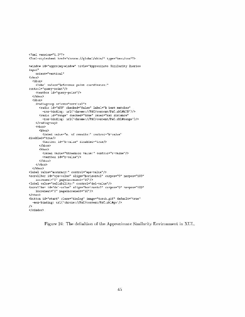
<?xml version="1.0"?>

<?xml-stylesheet href="chrome://global/skin/" type="text/css"?>

<window id="apprsimq-window" title="Approximate Similarity Queries

Input"

orient="vertical"

<vbox>

<hbox>

<label value="Reference point coordinates:"

control="query-point"/>

<textbox id="query-point"/>

</hbox>

<hbox>

<radiogroup orient="vertical">

<radio id="kNN" checked="false" label="k best matches"

-moz-binding: url('chrome://PAC/content/PAC.xbl#kNN')/>

<radio id="range" checked="true" label="max distance"

-moz-binding: url('chrome://PAC/content/PAC.xbl#range')/>

</radiogroup>

<vbox>

<hbox>

<label value="n. of results:" control="k-value"

disabled="true/>

<textbox id="k-value" disabled="true/>

</hbox>

<hbox>

<label value="threshold value:" control="r-value"/>

<textbox id="r-value"/>

</hbox>

</vbox>

</hbox>

<label value="accuracy:" control="eps-value"/>

<scrollbar id="eps-value" align="horizontal" curpos="0" maxpos="100"

increment="1" pageincrement="10"/>

<label value="reliability:" control="del-value"/>

<scrollbar id="del-value" align="horizontal" curpos="0" maxpos="100"

increment="1" pageincrement="10"/>

</vbox>

<button id="start" class="dialog" image="torch.gif" default="true"

-moz-binding: url('chrome://PAC/content/PAC.xbl#go'/>

/>

</window>

Figure 24: The de�nition of the Approximate Similarity Environment in XUL.

45

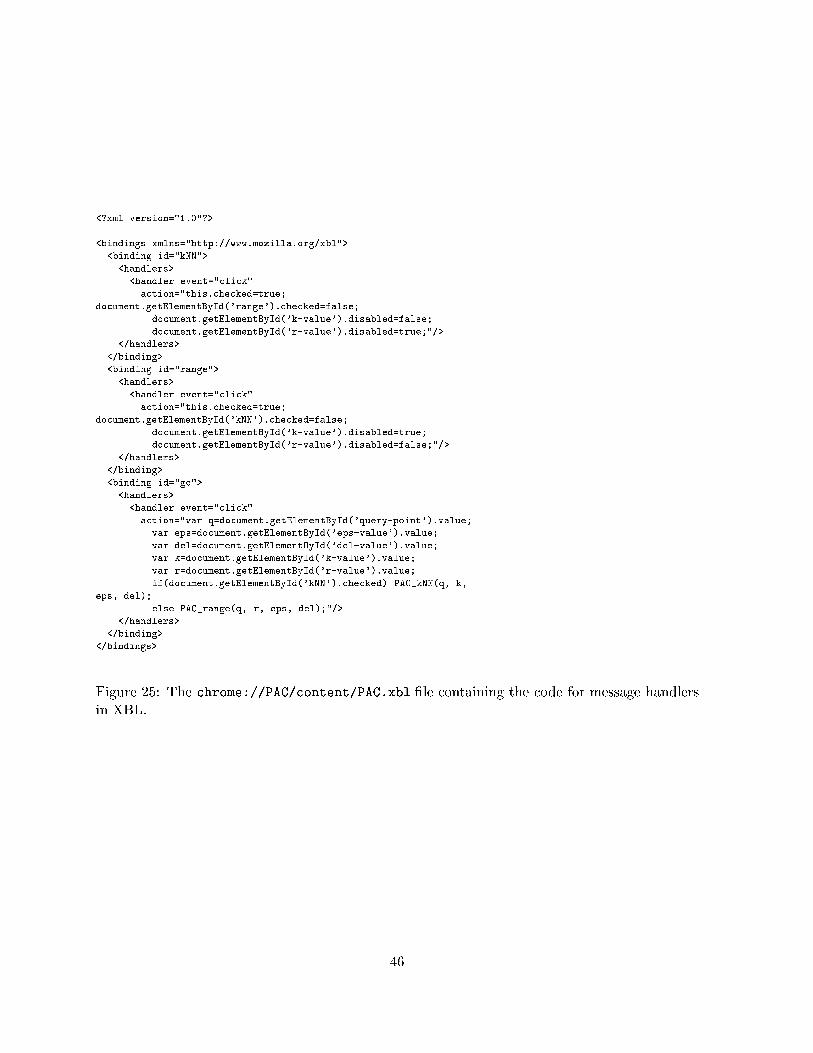
<?xml version="1.0"?>

<bindings xmlns="http://www.mozilla.org/xbl">

<binding id="kNN">

<handlers>

<handler event="click"

action="this.checked=true;

document.getElementById('range').checked=false;

document.getElementById('k-value').disabled=false;

document.getElementById('r-value').disabled=true;"/>

</handlers>

</binding>

<binding id="range">

<handlers>


action="this.checked=true;

document.getElementById('kNN').checked=false;

document.getElementById('k-value').disabled=true;

document.getElementById('r-value').disabled=false;"/>

</handlers>

</binding>

<binding id="go">

<handlers>


action="var q=document.getElementById('query-point').value;

var eps=document.getElementById('eps-value').value;

var del=document.getElementById('del-value').value;

var k=document.getElementById('k-value').value;

var r=document.getElementById('r-value').value;

if(document.getElementById('kNN').checked) PAC_kNN(q, k,

eps, del);

else PAC_range(q, r, eps, del);"/>

</handlers>

</binding>

</bindings>

Figure 25: The chrome://PAC/content/PAC.xbl �le containing the code for message handlers

in XBL.

46

Date post:	10-Feb-2017
Category:	Documents
Upload:	vandien
View:	215 times
Download:	1 times

Visual Data Mining system Architecture (Architettura del sistema ...

Documents