CESPRI Centro di Ricerca sui Processi di Innovazione e Internazionalizzazione

Università Commerciale “Luigi Bocconi” Via R. Sarfatti, 25 – 20136 Milano

Tel. 02 58363395/7 – fax 02 58363399 http://www.cespri.it

Stefano Breschi * Francesco Lissoni **

Mobility and Social Networks:

Localised Knowledge Spillovers Revisited WP n. 142 March 2003 ___________________________________ * Cespri, Dept. of Economics, Università “L. Bocconi”, Via Sarfatti 25, 20136 Milan (Italy) (e-mail: stefano.breschi@uni-bocconi.it).

** Dept. of Mechanical Engineering, Università di Brescia, via Branze 38, 25123 Brescia (Italy) (e-mail: lissoni@ing.unibs.it)

This research has been supported by a grant provided by the Italian Ministry for Research and University (MIUR). Seminar/conference participants at Cespri (Milan), UQAM University (Montreal) , Max-Planck Gesellschaft (Jena) and ZEW (Mannheim) have provided useful comments and suggestions. We are of course responsible for any remaining errors.. Jim Moody’s SPAN programme and SAS macros helped us at a crucial stage of data processing.

Abstract

The paper provides a reassessment of arguments and tests in support of the existence and

magnitude of localized knowledge spillovers proposed by Jaffe, Trajtenberg and Henderson

(1993). We use information in patents to control for the mobility of inventors across com-

panies and space, as well as for the network ties that such mobility helps establishing. Our

results indicate that localisation effects tend to vanish where citing and cited patents are not

linked to each other by any network relationship. On the contrary, knowledge flows, a s

evidenced by patent citations, are strongly localized to the extent that labour mobility and

network ties also are. We interpret these results as evidence that geography is not a suffi-

cient condition for accessing a local pool of knowledge, but it requires active participation

in a network of knowledge exchanges. Moreover, hiring workers from competitors and

other firms seems to be a key means to access such a network.

JEL Codes: O31, J60

Keywords: knowledge spillovers; localization; patent citations

1

1. Introduction

In the past few years, very few buzzwords have resonated, through economists’, geogra-

phers’, and policy-makers’ ears alike, more than “LKS”.

LKS stands for “Localized Knowledge Spillover”, an effective micro-founded, policy-ori-

ented rewording of Marshall’s classic metaphor on the secrets of industry being in the air.

By invoking the existence of LKSs, supporters of public plans for R&D funding can reas-

sure taxpayers that it will be the local community to reap most of the benefits of those

plans. The recipients of public funds (whether incentive-driven new private R&D facilities,

or local universities) will in fact produce some knowledge externalities. Any new knowledge

of that kind, however, will comprise a vast amount of skills, intuitions, and best practices,

whose transmission will require face-to-face contacts and lengthy explanations. As a result,

only local companies will manage to access that body of knowledge through frequent inter-

action with its sources, so that the ultimate result of the policy plan can be reassuringly de-

fined as the creation of a local public good.

Strong scientific support to such a thesis, and indeed a major diffusion drive to the LKS

acronym, has come from an engaging and extremely successful econometric research pro-

gramme, aimed at using patents, innovation counts, and patent citations as useful indicators

of the existence and geographical reach of knowledge externalities (for a survey: Feldman,

1999; for a few key collected essays: Jaffe and Trajtenberg, 2002).

This paper aims at contributing to that research programme, by adding both new data

(namely, data on Italian patents) and new measurable variables, such as social proximity be-

tween inventors, and inventors’ mobility across firms.

To do so, we first sum up the main features of the LKS research programme, and place

particular emphasis on the discussion of a statistical exercise first proposed by Jaffe, Tra-

jtenberg and Henderson (JTH) in 1993 (section 2). We then describe our data and meas-

urement techniques (section 3), and replicate that exercise, by adding our new variables

and commenting the results (section 4). In section 5, we conclude by setting out our plans

for further empirical research.

2

2. The LKS research programme

Although pioneered in its present form by Jaffe (1989), the LKS research programme is

possibly the last legacy from professor Zvi Griliches’ long-time efforts to produce reliable

methodologies for the estimation of the relationship between R&D and economic growth.

In order to test models of endogenous growth, those methodologies had to measure effec-

tively the extent of knowledge externalities, which in a production-function frame had to

take the form of R&D spillovers across firms and/or from universities and public labs to

firms. By regressing growth in per-capita income or total factor productivity against public

and private R&D expenditures, professor Griliches reached the conclusion that knowledge

spillovers existed and mattered a lot, but also that, in the absence of better data and im-

proved econometric techniques, his own and many others’ studies could not prove any-

thing more than “back-of-the-envelope” calculations (Griliches, 1992).

The main challenge consisted in disentangling “pecuniary externalities” and “pure spill-

overs”. The first ones are described as “R&D intensive inputs […] purchased at less than

their full ‘quality’ price”1 (we notice immediately that location advantages may well explain

the extent of the discount). The second ones are “ideas borrowed by research teams”2 of

one firm from the research results of another one.

By citing Jaffe’s early work (1986, 1988), prof. Griliches pointed out that a promising ap-

proach consisted in measuring separately the knowledge stock (e.g. the cumulated R&D) of

individual companies or universities (or, at a more aggregate level, industries), and then

weighing the influence of that stock on other companies’ knowledge output, as measured,

for example, by patents.

Weights had to be inversely related to the “distance” between “sending” and “receiving”

agents. Griliches (1992) mainly thought of “technological distance” measures, such as dif-

ferences in the technological base of firms and industries.

Jaffe (1989) coupled to technological differences a few measures for geographical distance.

The basic intuition behind that addition was the need to recognize the “tacit” nature of

knowledge, that is the need of frequent interaction between “sender” and “receiver” of the

1 Griliches, 1992; p. 36. 2 Griliches, 1992; p. 36.

3

spillover, in the form of face-to-face contacts between people working for the former and

people working for the latter.

Soon geographical distance took centre stage, possibly because of the renewed interest into

economic geography spurred by the success of Paul Krugman’s “Geography and Trade”

lectures (Krugman, 1991). Jaffe’s results, strengthened by similar, and similarly successful

exercises by Acs, Audretsch and Feldman3, were extremely timely in both confirming the

geographic dimension of a key economic activity such as innovation, and in challenging

Krugman’s provocative assessment of “Marshallian externalities of the third kind” (read:

knowledge spillovers) as both non-measurable and hardly conceivable as localized, and

therefore irrelevant to the economic analysis of industrial localization.

The definitive piece of work in dismantling Krugman’s contempt, and in popularizing LKS

even among the most econometric-phobic sects of POGs (“plain old geographers”, as in

David’s 1999), came two years later, by Jaffe, Trajtenberg, and Henderson (1993; from now

on JTH). They worked out an imaginative “controlled experiment”, specifically designed to

test for the localization of knowledge spillovers, as measured by patent citations.

Quite differently from previous, Griliches-style work, here patents are used outside any

“production function” frame; nor any R&D statistics are used, so that no strong assump-

tion on the way knowledge affects innovation (and from here, growth) is put forward. Still,

a few assumptions on the way knowledge “tacitness” may affect geography are retained

from earlier work.

We now turn to describe the experiment, and discuss critically those assumptions.

2.1 The JTH experiment: design and technicalities

The JTH’s experiment tests whether knowledge spillovers are indeed localized, and the ex-

tent of that localisation. To do so, a sample of patents applied for within a relatively short

span of time is taken4. Then, all citations of those patents by successive ones are consid-

ered, with the exclusion of self-citations, i.e. those citations running between two patents

assigned to the same company.

3 Key papers: Acs, Audretsch and Feldman (1992); Audretsch and Feldman (1996); Feldman and Florida (1994). More citations in Feldman (1999). 4 JTH selected two samples, one for 1975 and another for 1985, in order to check for changes in the geographical reach of spillovers due to changes in the patent contents, as a result of changes in patent rules and applicants’ attitudes

4

To the extent that those citations are not imposed by patent examiners, they are taken as

representative of some form of knowledge spillover from the inventors’ team behind the

cited patent to the team behind the citing one5. Moreover, to the extent that knowledge

spillovers are geographically localised, citations should come disproportionately from the

same geographical area as the cited patent.

However, this simple test would tell us little about the localisation of knowledge spillovers,

unless one controls for the pre-existing geographic concentration of innovative activities.

In other words, one might find that a disproportionate share of citations come from the

same area as the cited patent simply because the production of technological innovations (i.e.

patents) happens to be agglomerated in that area. The production of innovations, in turn,

may be spatially agglomerated for a number of reasons, which have nothing to do with the

access to the local knowledge pool and may be more properly categorised as “pecuniary”

externalities (e.g. availability of skilled labour and specialised inputs, the infrastructure

endowment of cities and regions, etc.).

The most important innovation of the JTH paper was to develop a methodology, which

allows one to separate the effects of ‘pure’ knowledge spillovers from the impact of other

agglomeration forces. Specifically, JTH built a control sample of patents in the following

way. Each citing patent was matched to a randomly drawn patent, which had the same

technology class and application date as its matched citing patent, but did not cite the same

originating patent6.

5 Current patent applications cite older ones in order to define what is called “prior art” and, by contrast with the their own contents, the extent of their novelty claim. Some citations may be inserted in the application by the inventors themselves, thus witnessing they benefited from some of the knowledge content of the cited patent. Many other citations, however, are added by patent examiners and/or the applicant’s patent consult-ants, for legal reasons. This type of citations have hardly anything to do with knowledge flows from the in-ventors of the cited patents to those of the citing one: much more likely, they reflect some duplication of the research efforts the inventors were unaware of. Duty of candour imposes USPO applicants to list all of the previous patents they are aware of, which can be considered prior art. EPO rules are much less strict in this sense, so that we expect the percentage of citations coming from examiners and consultants to be higher. Thus, our EPO data should be a poorer proxy of “true” knowledge flows than JTH’s USPO ones. Notice, however, that a high percentage of examiner-imposed citation should in principle dilute the localization ef-fect. 6 Patent offices classify applications according to very detailed codes, which should mirror the patent technological contents. JTH’s data fall under the US Classification (USC) system. Ours under the IPC (Inter-national Patent Classification) system. JTH matched patents according to the first three out of the nine digits of the USC. For a criticism of this choice, see Thompson and Fox-Kean (2002). Notice also that JTH’s data come from USPO, the US Patent Office where the first-to-invent rule applies: patents are applied for by in-ventors, who then assign them to their employer or whatever company they produced the invention for. In first-to-file systems such as the one followed by EPO, the European Patent Office, companies apply directly

5

Finally, cited, citing, and control patents were assigned to a geographical entity (local area,

state, country), according to the address of the inventor (if only one is credited on the pat-

ent document) or one of the many different addresses that may appear on patents credited

to a team of inventors7.

JTH’s experiment consisted then in comparing the frequency with which citing and cited

patents match geographically, with the frequency with which control and cited patents

match geographically. If the former turns out to be significantly greater than the latter, this

should interpreted as evidence of localisation effects (i.e. spillovers) over and above the

agglomeration effects arising from other sources. More specifically, the JTH exercise con-

sisted in comparing “the probability of a patent maching the originating patent by geo-

graphic area, conditional on its citing the originating patent, with the probability of a match

not conditioned on the existence of a citation link. This noncitation-conditioned probability gives a

baseline or reference value against which to compare the proportions of citations that

match” (JTH, 1993, p. 581). The evidence reported by JTH shows indeed that citations are

highly localised. Citing patents are up to two times more likely than the control patents to

come from the same state, and up to six times more likely to come from the same met-

ropolitan area.

2.2 Problems of interpretation and the need for further controls

JTH’s interpretation of their own results as evidence of the existence of pure spillovers

hides quite a naïve portrait of the channels along which knowledge externalities flow. Basi-

cally, one should believe that knowledge externalities are the result of oral communications.

Although no thorough discussion can be found in JTH, nor in any other econometric work

on LKS, many scattered remarks point in this direction (for a discussion and a few quotes,

see Breschi and Lissoni, 2001).

Within the original production-function frame that started the LKS research programme,

the naivety of the description comes as a logical necessity: any input-embodied knowledge

(whether the input is labour, or some good or service) is traded consciously between the

two sides of the market; as long as it is not entirely paid for, some externality may exist, but for patents in their names, and simply list the inventors’ names to oblige to the legal duty of making clear who, eventually, will be entitled to the so-called “equo premio”. 7 JTH’s rules in this case are quite complicated. Two full paragraphs of their article are devoted to their explanation, at page 585. States are the US ones, while country is registered as US vs. non-US. Local areas are identified by Metropolitan Areas, either taken from statistical classification or adjusted by JTH to the purposes of their paper.

6

of a pecuniary kind. Pure spillovers can take place only within the realm of trade-unrelated

personal communication, or through reverse engineering of some kind (i.e., reverse engi-

neering both of manufactured goods and of technical documents, such as patents).

As soon as “tacitness” is called in, to explain why distance matters, reverse engineering ex-

its the scene: studying thoroughly a piece of machinery or a patent is not enough to under-

stand how it works, unless the original inventors adds some explanation and/or practical

demonstration.

But why should that inventor accept to pass on information deliberately, without being

paid for? How can we make sure that short distances convey pure spillovers and not, once

again, pecuniary ones?

Social obligations are the answer. This is best seen when discussing knowledge flows from

universities to fi rms: treating those flows as pure spillovers sounds reasonable, since uni-

versity researchers obey to the principles of “Open Science” and dedicate themselves to the

production of public goods. They have the duty to communicate and discuss widely and

freely their results and discoveries. It is not by chance that LKS literature devotes special

attention to externalities from local universities.

Community of practitioners may also have some obligations of this kind. As described by

von Hippel (1987), industrial researchers and engineers working for different companies

within the same technological niche may be willing to provide their colleagues with free ad-

vice, with their employers tolerating this practice as long as it provides some returns in

terms of access to information.

At a closer look, however, one realizes that community of scientists or practitioners ex-

change “tacit” knowledge even from a long spatial distance, that is, they are not necessarily

concentrated in space. Meeting a few times a year, at conferences and workshops, may be

enough for two scientists to get mutual understanding, and start exchanging files, refer-

ences, and any other piece of information. As made clear by Cowan, David and Foray

(2000), the knowledge exchanged in that way is still “tacit”, to the extent that both oral and

written messages make use of a language and some basic concepts whose meaning is highly

context-specific and would take a long time to explain to outsiders. Scientists and industrial

researchers engaged in this kind of exchanges are producing knowledge which we can por-

trait as a club good (Cornes and Sandler, 1996).

7

Spatial closeness thus disappears as a necessary condition for setting up a club of this kind:

Fairchildren may all be located in Silicon Valley, but communities of open source software

developers are scattered worldwide.

Nor spatial closeness is a sufficient condition: no multinational can hope to set up a branch

plant within an Italian industrial district with the hope of being admitted to the tight web of

personal relationships that convey the local knowledge.

This is not to say that personal acquaintances and face-to-face contacts do not matter: on

the contrary, members of a social network who know each other personally exchange more

information and help, and do it more frequently; those with many acquaintances send and

receive more messages; and peripheral members, who are in touch with very few network

members are reached by news later than central actors, and meet more difficulties to un-

derstand and appreciate them. Above all, peripheral members who would like to be intro-

duced to some network member they have never met or interacted with, have to ask

around a lot before finding who can help them in that direction (who knows whom).

This means that, when thinking of knowledge as a club good, we can distinguish both be-

tween club members and outsiders, and between members at different social distances

from each other. Spillovers from an active club member will reach distant fellow members

with some delay or imprecision, and will possibly never reach outsiders.

It remains true, however, that many social networks dedicated to the production of knowl-

edge as a club good are geographically bounded, since spatial proximity may help the net-

work members to communicate more effectively and patrol each other’s behaviour (com-

pliance with the social norms of inward openness and outward secrecy).

We conclude that co-localization (spatial proximity) is used by JTH as a proxy for what so-

cial network analysis calls social proximity. To the extent that many networks are concen-

trated in space, co-localization would appear as a significant determinant of access to spill-

overs.

If this is true, by replacing co-localization with direct measurers of social proximity, we

would diminish the importance of geography as an explanatory variable of spillovers: the

latter would be localized (in the physical space) if and only if a significant proportion of so-

cial networks are also localized in space.

8

Proposing a measure of social proximity and showing its usefulness is the first contribution of this paper to

refining the JHT analysis. As explained with more details in the next section, we assume that

inventors who worked together on the same patent know each other well enough to be

willing to exchange information in future, and to tolerate to see that information passed on

to somebody else the receiver knows personally. That is, the clubs of researchers and tech-

nologists we consider relevant for our analysis are described as social network of inventors. To

the extent that these networks include members from more than one company, we expect

some knowledge to circulate freely among the various companies, the extent of which will

be measured by patent citations across firms.8

The second contribution of our paper to improving the JHT analysis consists in showing how many patent

citations come from “mobile inventors”, and how this result casts a few doubts on the capability of citations

to represent “pure” knowledge spillover. This criticism comes from the observation that, for social

networks of inventors to span across different firms, some inventors must move across

companies. Two inventors currently employed by different companies may be supposed to

know each other only if they previously worked together in the same company, or at most

in a joint venture between their current employers. This is also a reasonable guess on how

socializing among professionals actually occurs: industrial researchers who met only at

conferences, and have no personal acquaintances in common, can hardly exchange

sensitive information, or be willing to waste time to help each other. The opposite holds

for two former colleagues, one of which may also introduce the other to his new ones.

Here comes in a conceptual problem. Any inventor who moves from one company to an-

other one brings along some technical knowledge. To the extent that he can appropriate it,

any pure spillover disappears, and only pecuniary externalities survive. In other words, by

hiring an inventor, the new employer gets access to the specific knowledge embodied in the

inventor and to the social capital of contacts he brings with him. If the inventor is able to

fully appropriate the value of his knowledge and social capital, the externality is fully in-

ternalised. Moreover, even if the inventor cannot fully appropriate the value of his knowl-

8 One could argue that previous common working experiences are quite a narrow criterion to define personal acquaintances However, as we made clear above by recalling von Hippel’s and Cowan et al.’s work, it is only acquaintances among practitioners that matter: the receiver of the knowledge flow may be up to task of understanding it, which is not the case with acquaintances that have nothing to do with professional life. Notice also that since we measure flows with heavy technical contents, pure exchanges of broadly conceived new technical ideas (such as those that may take place between a scientist or technologist and an entrepreneur with no technical background) do not matter.

9

edge, only a pecuniary externality is likely to arise, i.e. the new employer gets access to a

fundamental knowledge input at a price lower than its full quality price.

Patent citations allow us to control for this possibility, or at least for its likelihood. Besides

company self-citations (one company’s patent cites a patent from the same company, as in

JTH) we can check for personal self-citations (one inventor’s patent cites a patent from the

same inventor, although the two patents belong to different companies).

A high rate of personal self-citations makes the interpretation of any JTH-style experiment

quite fuzzy. To the extent that a mobile inventor keep in touch with his former employers

(i.e. leaves some colleagues behind, who he still considers members of his social network)

personal self-citations may signal a pure spillover. But if firms can access to the club good

only by recruiting a network member, the latter’s wage will reflect the value of the service

he provides to his new employer. This is true for all network members: the network as a

whole regards knowledge as a public (club) good, but one whose returns from sale are to-

tally appropriated by the network as a whole. Rules of behaviour by the network members

amount to nothing more than barter of knowledge assets, aimed at sharing those returns as

fairly as possible.

Notice that labour mobility is quite likely to be limited in space, with classical explanations

being sunk costs for relocation and aversion to the risk of unemployment.

Notice also that even JTH concede that under a few circumstances the validity of citations

as indicators of knowledge spillovers is doubtful. They suggest that

“… a firm [may get] a patent on an invention and then contracts with another

firm to make some part of it, or a machine necessary to make it, or any other

aspect of the downstream development. It is possible that such a contractor

might later get a patent on a related technology. To the extent that the flow of

rents between these parties is governed by a complete contract, there could

conceivably be no externality running from the original inventor to the con-

tractor. If we now add to this hypothetical contract the assumption that such

contracted development is relatively likely to be localised, we have the potential for

the observed localisation of citations to be greater than the true localisation of knowledge spill-

overs”9

9 Jaffe, Trajtenberg and Henderson (1993), p. 583-4; italics added

10

What we are saying here is that complete contracts may also govern the recruitment of in-

ventors, and the related access to knowledge as a club good. While JTH suggests that their

own doubts refer to a very special case, which does not invalidate the overall meaning of

patent citations, we put forward the suggestion that our doubts refer on the contrary to a

very common case.

Summing up, we will show that localized spillovers from our data set are localized, and

then control for social proximity among inventors. After proving the importance of that

control, we will move on to show how much of that proximity is due to labour mobility.

3. Data selection, and the measurement of mobility and social distance

Our methodology for selecting the three samples of patents follows rather closely the one

developed by JTH (1993).10 For this study we have selected three cohorts of “originating”

patents, consisting respectively of 1987, 1988 and 1989 patent applications. In each cohort

we included all patent applications by Italian firms and institutions to the European Patent

Office (EPO), which received at least one subsequent citation by the end of 1996.11 The

1987 originating cohort contains 699 patents that had received a total of 1631 citations by

the end of 1996. The 1988 originating cohort contains 843 patents that had received a total

of 1784 citations by the end of 1996. The 1989 originating cohort contains 779 patents that

had received a total of 1615 citations by the end of 1996.

For each cohort of “originating” patents, we eliminated all applications that either received

citations only from foreign organisations, or whose applicant was an Italian organisation,

but did not report any Italian inventor.12 It must be pointed out that the choice of excluding

citations from foreign companies implies that our study investigates the extent of intra-na-

tional localisation of patent citations, and it is unable to say anything about the extent of

international localisation. This choice has been mainly dictated by data constraints, as the

10 Recently, Thompson and Fox-Kean (2002) have criticised the selection process proposed by JTH. Their main argument is that the level of technology aggregation adopted by JTH to match citing and control pat-ents is likely to induce spurious localisation effects. Although the results are surely interesting, we will stick to the original JTH basic methodology, in order to allow easier comparisons of results. 11 Patent applications made by individual inventors were excluded from the sample. 12 The nationality of inventors has been derived by the address reported in patent documents. It is worth pointing out that the share of patent applications by Italian organisations made exclusively by non-Italian inventors is negligible (around 2% for each cohort of originating patents). On the other hand, the share of originating patents receiving citations only from foreign organisations is high (around 60% for each cohort of originating patents).

11

inclusion of citations coming from foreign organisations would have implied the construc-

tion of the whole network of inventors (see below). At the same time, given that the basic

intuition behind the notion of localised knowledge spillovers is that the strength of spill-

overs should fade with distance, our choice should not have any effect upon the results.

For each originating patent, we then took all patents that subsequently cited them as prior

art. For the construction of the citing sample, we considered only patent applications made

before 1996 inclusive. Moreover, since we are interested in knowledge spillovers, we re-

moved all observations in which citing and originating patents have the same applicant (i.e.

self-citations).

Finally, from each citing patent we took the primary classification code at the 4-IPC-digit

level and used this to construct a sample of “control” patents. Specifically, for each citing

patent we identified all patents in the same patent class with the same application year. We

then chose from that set a control patent whose application date was as close as possible to

that of the citing patent, and that did not cite the same originating patent. The resulting

data set therefore consists of all “originating” patents, for which there is a matching of cit-

ing and control patents. In turn, each citing patent is paired with a specific control patent

within the same technological class and the with (approximately) the same application date.

The final sample consists of 366 originating patents, which have received 483 citations

from other Italian organisations.

3.1 Geographic assignment of patents

A major problem in measuring the frequency of matching by geographic area between cited

and citing (control) patents relates to the way patents are assigned to locations. Patent

documents report the town/city and postal address of each inventor. However, the prob-

lem is that patents can have multiple inventors. Therefore, the location of patents in geo-

graphic space cannot be resolved in a unequivocal way. In case of multiple inventors, JTH

assigned each patent to the country/state in which pluralities of inventors resided, with ties

assigned arbitrarily. Here, we take a slightly different approach and argue that two patents

match geographically to the extent that they share at least one inventor’s location in com-

mon.

12

3.2 Linkages: mobility and “social” distance

The major novelty of our study consists in improving the methodology described above

with the purpose of assessing the relative importance of pre-existing “linkages” among pat-

ents on the probability of a geographical match. By reporting the names, surnames, address

and company affiliation of each inventor, patent documents allow us to measure at least

one type of such “linkages”, namely those arising from the participation in a common

“team” of inventors. Moreover, as the composition of teams changes among patents and

over time, exploring the composition of teams and their evolution permits to reconstruct

the network of collaborative relationships linking inventors (and, through them, patents).

The following hypothetical example illustrates the main idea (see Figure 1). Let suppose to

have five patent applications (1 to 5) and four applicants (α, β, γ, δ ). Applicant α made two

applications (1,2), while applicants β , γ and δ one each. Patents have been produced by

thirteen distinct inventors (A to M). So, for example, patent 1 applied for by company α

has been produced by a team comprising inventors A, B, C, D and E. A reasonable as-

sumption to make at this point is that, due to the collaboration in a common research pro-

ject, the five inventors are “linked” to each other by some kind of knowledge relation. The

existence of such a linkage can be graphically represented by drawing an undirected arrow

between each pair of inventors, as in the bottom part of Figure 1. Repeating the same exer-

cise for each team of inventors, we end up with a map representing the network of linkages

among all inventors.13

Using the graph just described, we can derive measures of “connectedness” among pairs of

patents. In order to see how, we have first to make some observations:

i) one can measure the “distance” among pairs of inventors in the network, by calculat-

ing the so-called geodesic distance.

13 In the language of graph theory, the top part of the figure reports the affiliation network of patents, applicants and inventors. An affiliation network is a network in which actors (e.g. inven tors) are joined together by common membership to groups of some kind (e.g. patents). Affiliation networks can be represented as a graph consisting of two kinds of vertices, one representing the actors (e.g. inventors) and the other the groups (e.g. patents). In order to analyse the patterns of relations among actors, however, affiliation networks are often represented simply as unipartite (or one-mode) graphs of actors joined by undirected edges- two inventors who participated in the same patent, in our case, being connected by an edge (see bottom part of Figure 1). Please note that the position of nodes and the length of lines in the graph do not have any specific meaning.

13

Figure 1. Bipartite graph of patents and inventors

The geodesic distance is defined as the minimum number of edges that separate two

distinct inventors in the network14. In Figure 1, for example, inventors A and C have

geodesic distance equal to 1, whereas inventors A and H have distance 3. This means

that the linkage between them is mediated by two other actors (i.e. B and F). In other

terms, even though inventor A does not know directly inventor H, she knows who

(inventor B) knows who (inventor F) knows directly inventor H.

i) Inventors may belong to the same component or they may be located in discon-

nected components. A component of a graph can be defined as a subset of the entire

graph, such that all nodes included in the subset are connected through some path. In

Figure 1, for example, inventors A to K belong to the same component, whereas in-

ventors L and M belong to a different component. A pair of inventors belonging to

14 For this and the following technical terms from social network analysis: Wasserman and Faust (1994)

Inventors

Patents

γ α

d b a

�

c h f e

�

g j i

�

k

�

a

b c

e d

f

g

h

i

j k

β Applicants

�

δ

l

l

m

m

Top: Bipartite graph of applicants (α, β, γ, δ), patents (1 to 5) and inventors (A to M), with lines linking each patent to the respective inventors and applicants.

Bottom: the one-mode projection of the same network onto just inventors

14

two distinct components have distance equal to infinity (i.e. there is no path con-

necting them).

ii) Some inventors have an extraordinarily important role in connecting different

components. We call them “mobile” inventors. For example, in Figure 1, inventor F

worked for both company α and β , thus connecting the team of inventors (B,D )

with the team of inventors (H,I). Similarly, inventor G worked both for company α

and γ, thus connecting the team (B,D,F) with the team (I,J,K).

The next question is how using information derived from the network of inventors in or-

der to ascertain the existence of a “linkage” between citing (control) and cited patents, be-

sides the link arising from the citation (non-citation) itself. This is again illustrated by the

previous example. Let us include now in the picture a patent document citing a previous

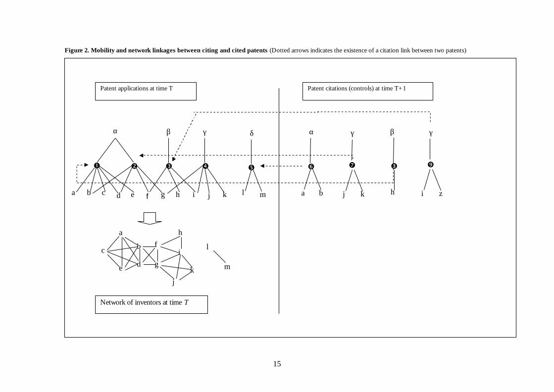
patent and not being a self-citation. Four sub-cases can arise (Figure 2):

1) There is no linkage between citing and cited patents. This is the case of patent 6

citing patent 5. Inventors of patent 6 (A,B) were not previously connected to

the inventors of patent 5 (L,M). They belonged to different components and

their distance was equal to infinity.

2) There is a direct linkage between citing and cited patents. This is the case of pat-

ent 7 citing patent 2. Inventors of patent 7 (J,K) know personally one of the in-

ventors of patent 2, namely inventor G, , through previous collaboration on

patent 4. At time T, they belong to the same connected component. Note that

the geodesic distance between either J or K and G is equal to 1. On the other

hand, the distance between either J or K and the ‘other’ inventors of patent 2

(B,D,F) is equal to 2.

3) There is an indirect linkage between citing and cited patents. This is the case of

patent 8 citing patent 1. Inventor of patent 8 (H) was not directly linked to any

of the inventors of patent 1 (A,B,C,D,E). However, she was indirectly linked to

them through collaboration with F on patent 3. In other words, inventor H

knows somebody (F) who knows inventors of patent 1. The geodesic distance

between H and any of the inventors of patent 1 is therefore equal to 2.

15

Figure 2. Mobility and network linkages between citing and cited patents (Dotted arrows indicates the existence of a citation link between two patents)

β

� �

γ α

d b a

�

c h fe

�

g j i

�

k

�

a

b c

e d

f

g

h

i

j k

β

�

δ

l

l

m

m

Patent applications at time T

Network of inventors at time T

Patent citations (controls) at time T+1

α

a b

γ

j k

�

h

�

γ

i z

16

4) There is a perfect linkage between citing and cited patents, when at least one in-

ventor appears in both patents. This is the case of patent 9 citing patent 3. One

of the inventors of patent 9 (I,Z) also appears in the team of inventors of pat-

ent 3 (I,F,H). The geodesic distance between I and herself is, by definition,

equal to 0. Note that the pair patent 9 – patent 3 is not a self-citation, as the

applicants of the two patents are different, and it should therefore be included

in the sample of originating patents. The linkage between citing and cited pat-

ents arises in this case from the mobility of one inventor (I) from company β to

company γ.

Using information from the pre-existing network of collaboration among inventors, we can

derive a measure of whether and to what extent citing (control) and cited patents are con-

nected by linkages other than the citation itself. Absent any linkage among the inventors of

the two patents, we can say that the latter are not connected. On the other hand, whenever

a linkage (direct, indirect, perfect) exists among the two patents, we can say that they are

connected.

3.3 Constructing the network of inventors

To implement the ideas described above, we have constructed a biographical dataset, based

upon all patent applications at the EPO from 1978 (its opening year) to 1999, which listed

at least one Italian inventor (the nationality being suggested by the inventor’s address). The

resulting database contains information on 30,170 inventors (name, surname, address) and

38,868 patent applications (technology classification code, name and address of the appli-

cant or grantee, application date and year). The number of inventors results after checking

raw data for misspelling of Italian personal and city names, use of initials, and loss of sec-

ond names. A round of e-mailing and phone calls helped identifying “mobile inventors”,

i.e. individuals with identical name and surname, but different postal addresses (and, possi-

bly, different company affiliations)15.

15 Inventors listed with the same name and surname (and different postal address) are identified as the same person when all or most of their patents belong to the same company: if this attribution sounds doubtful, further attempts of personal contacts have been made.

17

Table 1 – Evolution of the one-mode network of Italian inventors (1978-95)

Year Number of inventors

Number of edges (a)

Number of components of

size = 2 (b)

Average size of components (c)

Size of largest component (d)

1978-1986 6670 5203 1084 3.7 (8.0) 164

1978-1987 8058 6534 1287 3.8 (20.3) 723

1978-1988 9554 7912 1487 3.9 (26.9) 1032

1978-1989 11117 9557 1661 4.1 (33.4) 1359

1978-1990 12951 11474 1878 4.2 (43.7) 1885

1978-1991 14613 13294 2100 4.3 (48.1) 2194

1978-1992 16412 15421 2329 4.4 (52.6) 2504

1978-1993 18048 17514 2508 4.5 (58.0) 2858

1978-1994 19725 19437 2731 4.6 (61.7) 3166

1978-1995 21526 21593 2969 4.6 (64.8) 3449

(a) Total number of edges in the one-mode network of inventors (b) Number of components including at least two connected inventors (c) Average number of inventors in components with at least two inventors (standard deviation) (d) Number of inventors in the most numerous component

Using the data set just described, we have constructed the affiliation network of patents,

applicants and inventors, as well as the one-mode projection of the same network onto just

inventors, for each year from 1986 to 1995. Table 1 reports some descriptive statistics for

the resulting one-mode network of inventors. The network size grows as new inventors

start patenting. At the same time, the average number of inventors in each component also

grows, as previously disconnected teams are joined by some ‘mobile’ inventors. Notably,

also the absolute (and relative) size of the largest component grows steadily over time.

As explained above, we can derive measures of “linkage” between citing (control) and cited

patents using information provided by the inventors’ network. Specifically, for each pair of

citing-cited patents at time T (e.g. a patent issued in 1995 citing a patent issued in 1987), we

constructed the network of inventors at time T-1 (e.g. in 1994) and calculated the following

measures of “linkage”:

i) Connectedness: the variable takes value 1 if some of the inventors of citing and cited pat-

ents are in the same component at time T-1 (i.e. there is a path connecting at least two

of them); the variable takes value 0 in case the inventors belong to disconnected com-

ponents.

18

ii) Distance: the variable measures the shortest distance between the team of inventors of

the citing and the cited patent. The variable may take values comprised between 0 and

infinity. The distance between citing and cited patents is 0 when at least one inventor is

reported in both. The distance takes a positive and finite value when the two patents do

not share any inventor in common, but some of the inventors of citing and cited pat-

ents are in the same component at time T-1. Finally, the distance between the two pat-

ents is infinite when none of the inventors in the two teams belong to the same com-

ponent at time T-1.

The same variables are computed for each pair of control-cited patents. Table 2 reports the

composition of the final sample of patents, as well as some summary statistics concerning

the inventors included in it.

Table 2 – Sample of cited, citing and control patents: number of inventors and linkages

N. of patents

N. of inventors

N. of inv. per patent

N. of pairs (a)

N. of connected patents

Total (b) Geodesic = 0 (c) Geodesic = 1(c)

Cited 366 572 1.8 (1.2) -

Citing 483 721 2.0 (1.4) 1789 132 76 56

Control 483 726 1.9 (1.2) 1927 99 17 82 (a) A patent made by three inventors citing a patent made by two inventors generate 6 possible pairs of inventors, The

column reports the total number of pairs cited inventors – citing (control) inventors summed up over all patents in the sample.

(b) The column reports the absolute number of citing (control)-cited patents, whose inventors belong to the same con-nected component.

(c) The columns report the absolute number of citing (control) – cited patents, whose inventors have either 0 or a positive, but finite distance.

None but six of connected patents (both from the citing and the control sample) lists less

than two inventors. This suggests that inventor mobility is a phenomenon hardly distin-

guishable from social networking: it is not isolated inventors who move across companies,

but team workers, who meet and interact with different co-inventors when reaching the

new company. As a result of this interaction, even personal self-citation (i.e. self citation at

the inventor’s level) witness some knowledge diffusion, in this case from the mobile in-

ventors to new team mates

4. Results and comments

Table 3 reports the results of the JHT experiment, as run on our data. The first column re-

ports the percentage of citing patents that are co-located with the cited ones, at the city,

19

province or regional level16. The second column reports the same percentage for the

control sample, and the third one the “odds ratio” of a positive association between the

probability for a patent to be a citing and a co-located one. Odds ratio greater than one

signal that the differences between the values in the first and second columns are

significant, i.e. the existence of LKSs, according to the current interpretation of the JTH

experiment.17

It appears immediately that our data replicate successfully the JTH fundamental result: the

percentage of “co-located” citing patents is higher than expected, that is higher than the

equivalent percentage for control patents. In the Odds Ratio terminology, the probability

of co-location between a cited and a citing patent is much higher (OR>1) than the prob-

ability of co-location between the same cited patent and the “control” one.

Table 3 Co-location percentages, for citing and control patents

* 99% significant ; † 95% significant; ‡90% significant 16 Nomenclature of Statistical Territorial Units (NUTS) has been used here to define the spatial units of analysis. The city level corresponds to the so-called “comuni” (NUTS4), of which there are 8,100. Moreover, there are 95 provinces (NUTS3) and 20 regions (NUTS2). 17 A more user-friendly comparison technique of values in the first two columns would consist in computing t-tests for the difference in the frequency of geographical matching between, respectively, citing-cited patents and control-cited patents. JTH follow this strategy. Using odds ratios, however, turns useful for more com-plex comparisons, as those we propose below. Formally, we define odds ratios from the following 2x2 table whose row labels list the origin of the patent from either the “citing” sample or the “control” one (the two samples have the same size: 483 observations); the column labes tell us about the co -location of each patent and the cited one it refers to. For example, the cell p11 gives the probability of a patent being a citing one and being co -located with the cited patent.

Co-located? Yes Co-located? No Total Citing patent p11 p12 p11+p12=50 Control patent p21 p22 p21+p22=50 Total p11+p21=21.2 p12+p22=78.8 ? pij=100

The odds ratio for each table is then; OR = p11p22/p12p21 Odds ratios greater than one suggest a positive association between two probabilities, in our case the probability for a patent to come from the citing sample, and the probability of being co-located to the patent it cites.

Co-location percentages

Co-location level

Citing (n. of patents)

Control (n. of patents)

Odds Ratio (chi-square; df)

City 25.1 (121)

17.4 (84)

1.6 * (8.477; 1)

Province 38.7 (187)

29.8 (144)

1.5 * (8.498; 1)

Region 53.8 (260)

40.6 (196)

1.7 * (17.014; 1)

20

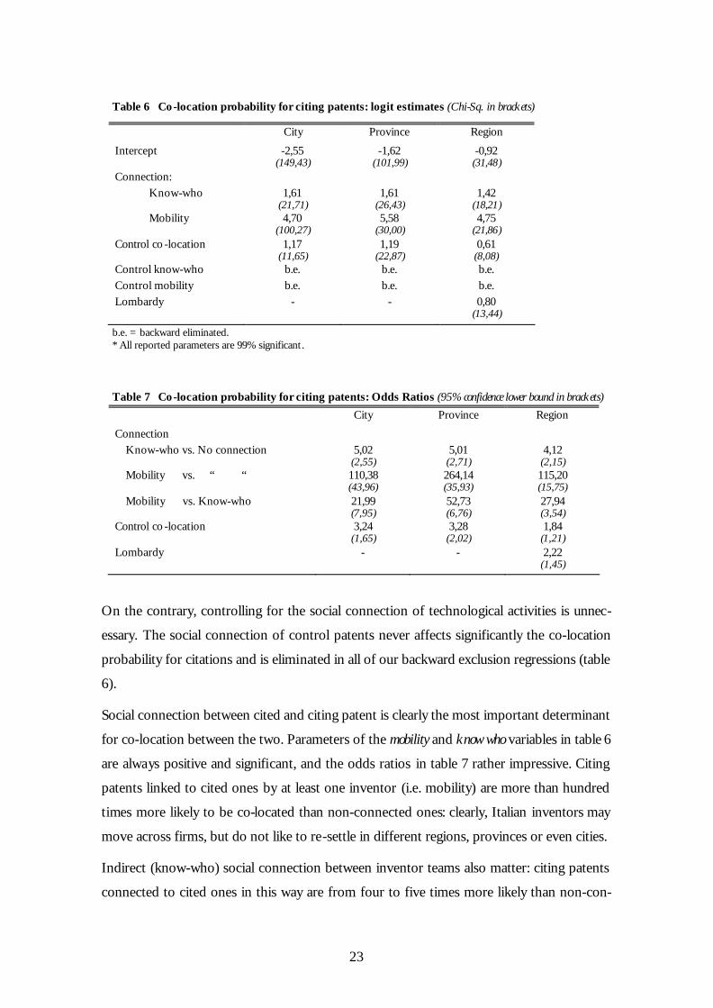
Tables 4 and 5 show the same kind of calculations, after controlling for social links among

the inventors. For each pair of patents (whether citing-cited or control-cited) we check

their “connectedness” value, and proceed to calculate again the co-location percentages for

citing and control patents (table 4).

We then move on to calculate different sets of “citation and co-location” Odds Ratios for

connected and non-connected pairs of patents. We then test homogeneity between the two

sets of Odds Ratios by calculating Breslow-Day statistics.

Finally, we apply Mantel-Haenszel methods to:

- performing a “nonzero correlation” test, which tells us whether some association

between “citation” and “co-location” survives to the adjustment for connectedness;

- calculating the lower-bound 95% confidence limit of so-called “common odds ra-

tios”: for any positive association between citation and co-location to be significant

this value must be higher than one.

Table 4 Co-location percentages, citing vs. control patents, adjusted for connectedness

Size of samples after adjusting for connectedness: Non-connected: 351 (citing) + 384 (control) Connected : 132 (citing) + 99 (control)

We first notice from table 4 that co-location percentages for non-connected patents,

whether from the citing or control sample, are much lower both of those for the aggregate

sample (see table 3) and of those for connected patents. The highest co-location for non-

connected patents come from analysis at the regional level of the citing sample, and it is

just 41 per cent, less than the minimum value for connected patents (44.4 per cent, from

city-level analysis of the control sample). This clearly suggests connectedness to bear great

influence on any result one can get from the spatial analysis of patent citations.

Table 4 also suggests that, in absence of any social connection with cited patents, citing and

control patents bear no differences in terms of co-location at the city and province level (at

Non-connected Connected

Co-location level

Citing (n. of patents)

Control (n. of patents)

Citing (n. of patents)

Control (n. of patents)

City 8.8 (31)

10.4 (40)

68.2 (90)

44.4 (44)

Province 22.2 (78)

22.4 (86)

82.6 (109)

58.6 (58)

Region 41.0 (144)

33.3 (128)

87.9 (116)

68.7 (68)

21

the city level, control patents are indeed slightly more located than citing ones). Some dif-

ference may possibly survive at the regional level. On the contrary, when social connection

is present, JTH’s results survive at all levels.

These suggestions are confirmed by Odds Ratio analysis in table 5. “Citation and co-loca-

tion” Odds Ratios are always higher for connected patents than for non-connected ones, as

confirmed by the Breslow-Day test (differences between Odds Ratios for the two sub-

samples are always non homogenous). The same test and a look at the data, however, con-

firms those differences to be slightly less significant at the regional level, compared to

smaller geographical aggregates. Notice also that Odds Ratios for connected patents are

much higher than those calculated for all patents, while the opposite holds for non-con-

nected patents. Again, social connection is a pre-requisite for JTH’s results to survive, and

indeed be strengthened.

Table 5 Odds ratios for “citation and co-location”, for connected vs non-connected patents

* 99% significant ; † 95% significant; ‡90% significant

Nonzero correlation tests suggest the overall association between citation and co-location

to be weakened by the inclusion of controls for connectedness, with the usual exception of

regional level analysis. Similarly, the 95% lower bound limit for Odds Ratios include value

one for analysis at the city level, and barely excludes it for the province level.

As suggested in section 3, however, “connectedness” hides two fundamentally different va-

rieties of social links: those directly generated by the mobility of inventors, which reduces

the geodesic distance between two connected patents to zero, and those due to indirect

links between the teams of inventors, such that the distance is finite, but never less than

one (in particular, see table 2 and related comments).

Odds Ratio (chi-square; df)

Co-location level

Non-Connected

Connected Breslow-Day: Chi-sq./ df

Non-zero corr: Chi-sq. / df

Common OR 95%: confidence limit

City 0.8 (0.528; 1)

2.7 * (13.086; 1)

9.930 / 1 * 3.707 / 1 ‡ 0.991

Province 0.9 (0.003; 1)

3.3 * (16.255; 1)

12.066 / 1 * 4.065 / 1 † 1.006

Region 1.4 † (4.655; 1)

3.3 * (12.857; 1)

5.387 / 1 † 11.980 / 1 * 1.228

22

In order to test the effects of these two varieties of social links, we run a series of logit re-

gressions of the same kind one can find in JTH18. Only patents from the citing sample are

considered, with the binary variable “co-location” (yes/no) as the dependent one. Explana -

tory variables are just three. The first one refers to connectedness, and distinguishes be-

tween connectedness from “mobility” and “know-who” connectedness, due to direct or indi-

rect social links between inventors from the two patents’ teams, but no overlapping be-

tween the two; no connectedness take the zero (baseline) value. The second one controls

for the co-location of technological activities, and makes use once again of information

from the control sample: for each citing patent, it takes value one if the related control pat-

ent is co-located with the cited one, and zero otherwise (control co-location). Finally, we also

control for the likelihood of patent connection by technological field, that is we control

whether the control and cited patents are linked by mobility or know-who connections, or

are not connected at all (control mobility and control know-who)

We run backward-inclusion regressions for main effects only, starting with the inclusion of

all the explanatory variables. One regression is run for each geographical level. When it

comes to regional analysis we added a dummy variable for Lombardy, that is for the possi-

bility that at least one of the inventor of the cited patent points to Lombardy, the largest

and most innovative region of Italy, where more than 50 percent of the inventors come

from. Besides improving the estimates, this dummy is expected to cast light on the differ-

ent results we got in tables 4 and 5 for analysis at the regional level, as opposed to city- and

province-level analysis.

Tables 6 reports the results of the regressions, in terms of parameter estimation. Table 7

calculate the Odds Ratios one can derive from those parameters.

The importance of controlling for the localization of technological activities is confirmed:

the co-location of control patents bears always a positive influence (table 6) and the odds

that citations will be co-localized along with control patents are always greater than one

(table 7).

18 Jaffe, Trajtenberg and Henderson (1993), table IV, p. 593

23

Table 6 Co-location probability for citing patents: logit estimates (Chi-Sq. in brackets)

b.e. = backward eliminated. * All reported parameters are 99% significant.

Table 7 Co-location probability for citing patents: Odds Ratios (95% confidence lower bound in brackets)

On the contrary, controlling for the social connection of technological activities is unnec-

essary. The social connection of control patents never affects significantly the co-location

probability for citations and is eliminated in all of our backward exclusion regressions (table

6).

Social connection between cited and citing patent is clearly the most important determinant

for co-location between the two. Parameters of the mobility and know who variables in table 6

are always positive and significant, and the odds ratios in table 7 rather impressive. Citing

patents linked to cited ones by at least one inventor (i.e. mobility) are more than hundred

times more likely to be co-located than non-connected ones: clearly, Italian inventors may

move across firms, but do not like to re-settle in different regions, provinces or even cities.

Indirect (know-who) social connection between inventor teams also matter: citing patents

connected to cited ones in this way are from four to five times more likely than non-con-

City Province Region

Intercept -2,55 (149,43)

-1,62 (101,99)

-0,92 (31,48)

Connection: Know-who 1,61

(21,71) 1,61

(26,43) 1,42

(18,21) Mobility 4,70

(100,27) 5,58

(30,00) 4,75

(21,86) Control co -location 1,17

(11,65) 1,19

(22,87) 0,61 (8,08)

Control know-who b.e. b.e. b.e. Control mobility b.e. b.e. b.e. Lombardy - - 0,80

(13,44)

City Province Region

Connection Know-who vs. No connection 5,02

(2,55) 5,01 (2,71)

4,12 (2,15)

Mobility vs. “ “ 110,38 (43,96)

264,14 (35,93)

115,20 (15,75)

Mobility vs. Know-who 21,99 (7,95)

52,73 (6,76)

27,94 (3,54)

Control co -location 3,24 (1,65)

3,28 (2,02)

1,84 (1,21)

Lombardy - - 2,22 (1,45)

24

nected ones to be co-located. However, indirect links bear much less influence than mobil-

ity of inventors: besides comparing the two sets of Odds Ratios, one can also calculate

Odds Ratios for “mobility” vs. “know-who” connection, and notice that the former kind

of connection makes co-location probability at least 20 times more likely than the other.

Finally, we notice that the persistence of regional effects in tables 4 to 5 is not due to any

specific contribution of “unconnected” LKSs, but only to the peculiarity of the Italian in-

novation system, which is largely concentrated in Lombardy. The control variable for the

location of cited patents in this region is positive and significant, so that citations directed

to patents from Lombardy are two times more likely than others to be located in the same

region.

5. Conclusions

This paper brought JTH’s recommendation to use patent citations as “a paper trail” for

tracking knowledge flows to its extreme consequences. Patents have been used to check for

the mobility of inventors across companies and in space, as well as for the social ties that

such mobility helps establishing.

By doing so, we have given further confirmation to the original intuition of those econo-

mists and sociologists that first stressed the tacit content of technological knowledge:

knowledge always travel along with people who master it. If those people move away from

where they originally learnt, researched, and delivered their inventions, knowledge will dif-

fuse in space. Otherwise, access to it will remain constrained in bounded locations. That is,

knowledge flows (whether pure spillovers or traded services) are localized to the extent that

labour mobility also is.

Whether knowledge flows as measured by patent citation can represent “spillovers” or not

remains a matter for further enquiries. However, the overwhelming weight of mobility-in-

duced citations in our data casts some doubt on enthusiastic interpretation of JTH-linked

results as evidence of LKSs. Our intuition is that mobile inventors are most likely to be

scientific or technological “stars” whose wages or fees pay for the access they can provide

to a valuable club good such as the knowledge stock mastered by them, and the inventors

in their network. If it is so, either externalities may be fully internalised or just pecuniary

25

externalities arise (stars can accept lower wages and fees to the extent that their employees

and customers do not ask them to relocate), but no pure spillovers.

If confirmed, this interpretation bears great relevance for policy. It suggests that fashion-

able policies for attracting high-tech companies, private R&D facilities, and public R&D

funds in cities and regions, which are lagging behind the technological frontier may be fa-

tally flawed. Even if enough incentives would convince a few bright inventors to relocate,

these would maintain their social ties with distant colleagues and fellow researchers, and

find no reason to forge some new ones locally. Many more incentives would be then

needed for helping local firms to recruit those bright inventors, and finally get access to the

club good they can provide.

To confirm these conclusions, however, more empirical work is required. First, we will in-

crease our sample sizes, to allow for a more secure scrutiny of our results on Italian data.

Second, testing our hypothesis against USPO data, rather than EPO ones, could be more

safe, due to the greater accuracy with which the US Patent Office checks the information

provided by applicants on inventors. Finally, we ought to test our hypothesis on a larger,

and less peripheral, innovation system than the Italian one: in this way, we could generalize

our results.

While the first proposed extension will be a matter for further drafts of this paper, the oth-

ers will require separate efforts for setting up new data sets.

26

References

Acs Z.J., Audretsch D.B, Feldman M.P. (1992), “Real effects of academic research:

Comment”, American Economic Review 82 (1), 363-367.

Almeida P., Kogut B. (1999), “Localisation of knowledge and the mobility of engineers in

regional networks”, Management Science, 45(7), 905-917.

Audretsch D.B., Feldman M.P. (1996), “R&D spillovers and the geography of innovation

and production”, American Economic Review 86(3), 630-640

Breschi S., Lissoni F. (2001), “Knowledge Spillovers and Local Innovation Systems: A

Critical Survey”, Industrial and Corporate Change, vol. 10 n. 4, 975-1005.

Cornes R., Sandler T. (1996), The theory of externalities, public goods and club goods , Cambridge

University Press, Cambridge MA

David P.A. (1999), “Krugman's Economic Geography of Development. NEGs, POGs and

Naked Models in Space”, International Regional Science Review 22, 162-172

Feldman M.P. (1999), “The New Economics of Innovation, Spillovers and Agglomeration:

A Review of Empirical Studies”, Economics of Innovation and New Technology 8, pp.5-25.

Feldman M.P., Florida R. (1994), “The geographic sources of innovation: technological

infrastructure and product innovation in the United States”, Annals of the Association of

American Geographers 84(2), 210-229.

Griliches Z. (1992), “The Search for R&D Spillovers”, Scandinavian Journal of Economics 94,

Supplement, 29-47.

Jaffe A.B. (1986) “Technological opportunity and spillovers from R&D: Evidence from

firms’ patents profits and market value”, American Economic Review 76, 984-1001.

Jaffe A.B. (1988) “Demand and supply influences in R&D intensity and productivity

growth”, Review of Economics and Statistics LXX, 431-37.

Jaffe A.B. (1989), “Real effects of academic research”, American Economic Review 79, 957-70.

Jaffe A.B., Trajtenberg M. (2002) Patents, Citations, and Innovations : A Window on the Knowledge

Economy, MIT Press

Jaffe A.B., Trajtenberg M., Fogarty M.S. (2000), “Knowledge spillovers and patent cita-

tions: Evidence form a survey of inventors”, American Economic Review 90(2), 215-218.

27

Jaffe A.B., Trajtenberg M., Henderson R. (1993), “Geographic localisation of knowledge

spillovers as evidenced by patent citations”, Quarterly Journal of Economics 10, 577-598.

Krugman P. (1991), Geography and Trade, MIT Press, Cambridge MA.

Newman M.E.J. (2000), “Who is the best connected scientists? A study of scientific coau-

thorship networks”, SFI Working Paper 00-12-64, Santa Fe.

Newman M.E.J. (2001), “The structure of scientific collaboration networks”, Proceedings of

the National Academy of Science USA 98, 404-409.

Thompson P., Fox-Kean M. (2002), “Can Patent Citations Identify Knowledge Spillovers?”,

http://www.andrew.cmu.edu/~pt/current/working_papers.html, Carnegie Mellon

University

von Hippel E. (1987), “Cooperation Between Rivals: Informal Know-How Trading”, Re-

search Policy 16, 291-302.

Wasserman S., Faust C. (1994), Social Network Analysis: Methods and Applications, Cambridge

University Press.

Zucker L.G., Darby M.R., Armstrong J. (1998), “Geographically localised knowledge: spill-

overs or markets?”, Economic Inquiry 36(January), 65-86.